Observational Datasets Used in Climate Studies
Climate Datasets
Observations, including those from satellites, mobile platforms, field campaigns, and ground-based networks, provide the basis of knowledge on many temporal and spatial scales for understanding the changes occurring in Earth’s climate system. These observations also inform the development, calibration, and evaluation of numerical models of the physics, chemistry, and biology being used in analyzing past changes in climate and for making future projections. As all observational data collected by support from Federal agencies are required to be made available free of charge with machine readable metadata, everyone can access these products for their personal analysis and research and for informing decisions. Many of these datasets are accessible through web services.
Many long-running observations worldwide have provided us with long-term records necessary for investigating climate change and its impacts. These include important climate variables such as surface temperature, sea ice extent, sea level rise, and streamflow. Perhaps one of the most iconic climatic datasets, that of atmospheric carbon dioxide measured at Mauna Loa, Hawai‘i, has been recorded since the 1950s. The U.S. and Global Historical Climatology Networks have been used as authoritative sources of recorded surface temperature increases, with some stations having continuous records going back many decades. Satellite radar altimetry data (for example, TOPEX/JASON1 & 2 satellite data) have informed the development of the University of Colorado’s 20+ year record of global sea level changes. In the United States, the USGS (U.S. Geological Survey) National Water Information System contains, in some instances, decades of daily streamflow records which inform not only climate but land-use studies as well. The U.S. Bureau of Reclamation and U.S. Army Corp of Engineers have maintained data about reservoir levels for decades where applicable. Of course, datasets based on shorter-term observations are used in conjunction with longer-term records for climate study, and the U.S. programs are aimed at providing continuous data records. Methods have been developed and applied to process these data so as to account for biases, collection method, earth surface geometry, the urban heat island effect, station relocations, and uncertainty (e.g., see Vose et al. 2012;1 Rennie et al. 2014;2 Karl et al. 20153 ).
Even observations not designed for climate have informed climate research. These include ship logs containing descriptions of ice extent, readings of temperature and precipitation provided in newspapers, and harvest records. Today, observations recorded both manually and in automated fashions inform research and are used in climate studies.
The U.S Global Change Research Program (USGCRP) has established the Global Change Information System (GCIS) to better coordinate and integrate the use of federal information products on changes in the global environment and the implications of those changes for society. The GCIS is an open-source, web-based resource for traceable global change data, information, and products. Designed for use by scientists, decision makers, and the public, the GCIS provides coordinated links to a select group of information products produced, maintained, and disseminated by government agencies and organizations. Currently the GCIS is aimed at the datasets used in Third National Climate Assessment (NCA3) and the USGCRP Climate and Health Assessment. It will be updated for the datasets used in this report (The Climate Science Special Report, CSSR).
Temperature and Precipitation Observational Datasets
For analyses of surface temperature or precipitation, including determining changes over the globe or the United States, the starting point is accumulating observations of surface air temperature or precipitation taken at observing stations all over the world, and, in the case of temperature, sea surface temperatures (SSTs) taken by ships and buoys. These are direct measurements of the air temperature, sea surface temperature, and precipitation. The observations are quality assured to exclude clearly erroneous values. For temperature, additional analyses are performed on the data to correct for known biases in the way the temperatures were measured. These biases include the change to the observations that result from changes in observing practices or changes in the location or local environment of an observing station. One example is with SSTs where there was a change in practice from throwing a bucket over the side of the ship, pulling up seawater and measuring the temperature of the water in the bucket to measuring the temperature of the water in the engine intake. The bucket temperatures are systematically cooler than engine intake water and must be corrected.
For evaluating the globally averaged temperature, data are then compared to a long-term average for the location where the observations were taken (e.g., a 30-year average for an individual observing station) to create a deviation from that average, commonly referred to as an anomaly. Using anomalies allows the spatial averaging of stations in different climates and elevations to produce robust estimates of the spatially averaged temperature or precipitation for a given area. To calculate the temperature or precipitation for a large area, like the globe or the United States, the area is divided into “grid boxes” usually in latitude/longitude space. For example, one common grid size has 5° x 5° latitude/longitude boxes, where each side of a grid box is 5° of longitude and 5° of latitude in length. All data anomalies in a given grid box are averaged together to produce a gridbox average. Some grid boxes contain no observations, but nearby grid boxes do contain observations, so temperatures or precipitation for the grid boxes with no observations are estimated as a function of the nearby grid boxes with observations for that date.
Calculating the temperature or precipitation value for the larger area, either the globe or the United States, is done by averaging the values for all the grid boxes to produce one number for each day, month, season, or year resulting in a time series. The time series in each of the grid boxes are also used to calculate long-term trends in the temperature or precipitation for each grid box. This provides a picture of how temperatures and precipitation are changing in different locations.
Evidence for changes in the climate of the United States arises from multiple analyses of data from in situ, satellite, and other records undertaken by many groups over several decades. The primary dataset for surface temperatures and precipitation in the United States is nClimGrid,4 , 5 though trends are similar in the U.S. Historical Climatology Network, the Global Historical Climatology Network, and other datasets. For temperature, several atmospheric reanalyses (e.g., 20th Century Reanalysis, Climate Forecast System Reanalysis, ERA-Interim, and Modern Era Reanalysis for Research and Applications) confirm rapid warming at the surface since 1979, with observed trends closely tracking the ensemble mean of the reanalyses.1 Several recently improved satellite datasets document changes in middle tropospheric temperatures.6 ,7 ,8 Longer-term changes are depicted using multiple paleo analyses (e.g., Wahl and Smerdon 2012;9 Trouet et al. 201310 ).
Satellite Temperature Datasets
A special look is given to the satellite temperature datasets because of controversies associated with these datasets. Satellite-borne microwave sounders such as the Microwave Sounding Unit (MSU) and Advanced Microwave Sounding Unit (AMSU) instruments operating on NOAA polar-orbiting platforms take measurements of the temperature of thick layers of the atmosphere with near global coverage. Because the long-term data record requires the piecing together of measurements made by 16 different satellites, accurate instrument intercalibration is of critical importance. Over the mission lifetime of most satellites, the instruments drift in both calibration and local measurement time. Adjustments to counter the effects of these drifts need to be developed and applied before a long-term record can be assembled. For tropospheric measurements, the most challenging of these adjustments is the adjustment for drifting measurement time, which requires knowledge of the diurnal cycle in both atmospheric and surface temperature. Current versions of the sounder-based datasets account for the diurnal cycle by either using diurnal cycles deduced from model output11 ,12 or by attempting to derive the diurnal cycle from the satellite measurements themselves (an approach plagued by sampling issues and possible calibration drifts).13 ,14 Recently a hybrid approach has been developed, RSS Version 4.0,6 that results in an increased warming signal relative to the other approaches, particularly since 2000. Each of these methods has strengths and weaknesses, but none has sufficient accuracy to construct an unassailable long-term record of atmospheric temperature change. The resulting datasets show a greater spread in decadal-scale trends than do the surface temperature datasets for the same period, suggesting that they may be less reliable. Figure A.1 shows annual time series for the global mean tropospheric temperature for some recent versions of the satellite datasets. These data have been adjusted to remove the influence of stratospheric cooling.15 Linear trend values are shown in Table A.1.
Figure 1
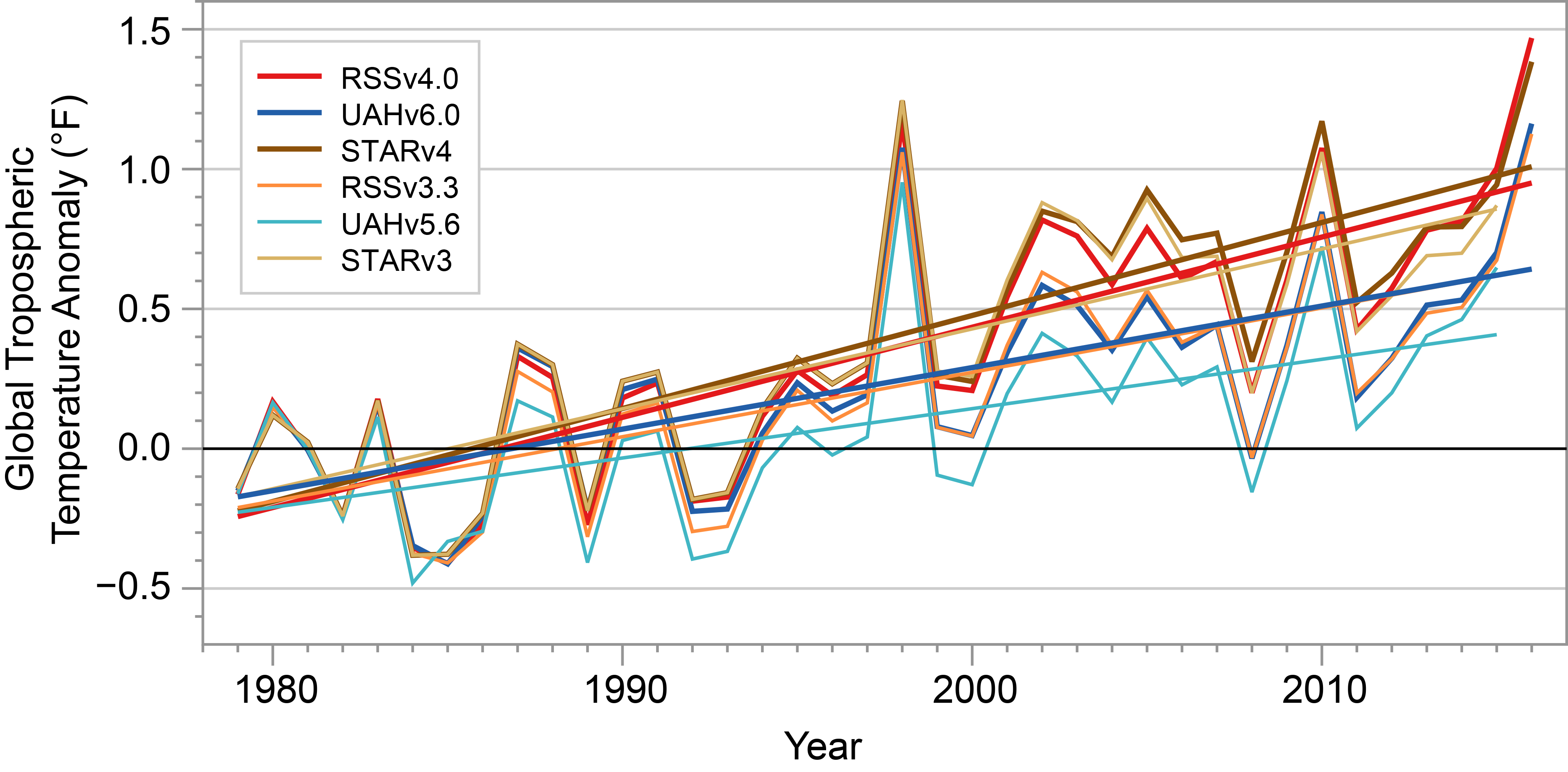
Annual global (80°S–80°N) mean time series of tropospheric temperature for five recent datasets (see below). Each time series is adjusted so the mean value for the first three years is zero. This accentuates the differences in the long-term changes between the datasets. (Figure source: Remote Sensing Systems).
| Dataset | Trend (1979–2015) (°F/Decade) | Trend (2000–2015) (°F/Decade) |
|---|---|---|
| RSS V4.0 | 0.301 | 0.198 |
| UAH V6Beta5 | 0.196 | 0.141 |
| STAR V4.0 | 0.316 | 0.157 |
| RSS V3.3 | 0.208 | 0.105 |
| UAH V5.6 | 0.176 | 0.211 |
| STAR V3.0 | 0.286 | 0.061 |
DATA SOURCES:
All Satellite Data are “Temperature Total Troposphere” time series calculated from TMT and TLS
(1.1*TMT) - (0.1*TLS). This combination reduces the effect of the lower stratosphere on the tropospheric temperature. (Fu, Qiang et al. "Contribution of stratospheric cooling to satellite-inferred tropospheric temperature trends." Nature 429.6987 (2004): 55-58.)
UAH. UAH Version 6.0Beta5. Yearly (yyyy) text files of TMT and TLS are available from
https://www.nsstc.uah.edu/data/msu/v6.0beta/tmt/
https://www.nsstc.uah.edu/data/msu/v6.0beta/tls/
Downloaded 5/15/2016.
UAH. UAH Version 5.6. Yearly (yyyy) text files of TMT and TLS are available from
http://vortex.nsstc.uah.edu/data/msu/t2/
http://vortex.nsstc.uah.edu/data/msu/t4/
Downloaded 5/15/2016.
RSS. RSS Version 4.0.
ftp://ftp.remss.com/msu/data/netcdf/RSS_Tb_Anom_Maps_ch_TTT_V4_0.nc
Downloaded 5/15/2016
RSS. RSS Version 3.3.
ftp://ftp.remss.com/msu/data/netcdf/RSS_Tb_Anom_Maps_ch_TTT_V3.3.nc
Downloaded 5/15/2016
NOAA STAR. Star Version 3.0.
ftp://ftp.star.nesdis.noaa.gov/pub/smcd/emb/mscat/data/MSU_AMSU_v3.0/Monthly_Atmospheric_Layer_Mean_Temperature/Merged_Deep-Layer_Temperature/NESDIS-STAR_TCDR_MSU-AMSUA_V03R00_TMT_S197811_E201709_C20171002.nc
ftp://ftp.star.nesdis.noaa.gov/pub/smcd/emb/mscat/data/MSU_AMSU_v3.0/Monthly_Atmospheric_Layer_Mean_Temperature/Merged_Deep-Layer_Temperature/NESDIS-STAR_TCDR_MSU-AMSUA_V03R00_TLS_S197811_E201709_C20171002.nc
Downloaded 5/18/2016.
References
- Christy, J. R., R. W. Spencer, W. B. Norris, W. D. Braswell, and D. E. Parker, 2003: Error estimates of version 5.0 of MSU–AMSU bulk atmospheric temperatures. Journal of Atmospheric and Oceanic Technology, 20, 613–629, doi:10.1175/1520-0426(2003)20<613:EEOVOM>2.0.CO;2. ↩
- Fu, Q., and C. M. Johanson, 2005: Satellite-derived vertical dependence of tropical tropospheric temperature trends. Geophysical Research Letters, 32, L10703, doi:10.1029/2004GL022266. ↩
- Karl, T. R., A. Arguez, B. Huang, J. H. Lawrimore, J. R. McMahon, M. J. Menne, T. C. Peterson, R. S. Vose, and H.-M. Zhang, 2015: Possible artifacts of data biases in the recent global surface warming hiatus. Science, 348, 1469–1472, doi:10.1126/science.aaa5632. ↩
- Mears, C. A., and F. J. Wentz, 2009: Construction of the Remote Sensing Systems V3.2 atmospheric temperature records from the MSU and AMSU microwave sounders. Journal of Atmospheric and Oceanic Technology, 26, 1040–1056, doi:10.1175/2008JTECHA1176.1. ↩
- Mears, C. A., and F. J. Wentz, 2016: Sensitivity of satellite-derived tropospheric temperature trends to the diurnal cycle adjustment. Journal of Climate, 29, 3629–3646, doi:10.1175/JCLI-D-15-0744.1. ↩
- Po-Chedley, S., T. J. Thorsen, and Q. Fu, 2015: Removing diurnal cycle contamination in satellite-derived tropospheric temperatures: Understanding tropical tropospheric trend discrepancies. Journal of Climate, 28, 2274–2290, doi:10.1175/JCLI-D-13-00767.1. ↩
- Rennie, J. J. et al., 2014: The international surface temperature initiative global land surface databank: Monthly temperature data release description and methods. Geoscience Data Journal, 1, 75–102, doi:10.1002/gdj3.8. ↩
- Spencer, R. W., J. R. Christy, and W. D. Braswell, 2017: UAH Version 6 global satellite temperature products: Methodology and results. Asia-Pacific Journal of Atmospheric Sciences, 53, 121–130, doi:10.1007/s13143-017-0010-y. ↩
- Trouet, V., H. F. Diaz, E. R. Wahl, A. E. Viau, R. Graham, N. Graham, and E. R. Cook, 2013: A 1500-year reconstruction of annual mean temperature for temperate North America on decadal-to-multidecadal time scales. Environmental Research Letters, 8, 024008, doi:10.1088/1748-9326/8/2/024008. ↩
- Vose, R. S., D. Arndt, V. F. Banzon, D. R. Easterling, B. Gleason, B. Huang, E. Kearns, J. H. Lawrimore, M. J. Menne, T. C. Peterson, R. W. Reynolds, T. M. Smith, C. N. Williams, and D. L. Wuertz, 2012: NOAA’s Merged Land-Ocean Surface Temperature Analysis. Bulletin of the American Meteorological Society, 93, 1677–1685, doi:10.1175/BAMS-D-11-00241.1. ↩
- Vose, R. S., M. Squires, D. Arndt, I. Durre, C. Fenimore, K. Gleason, M. J. Menne, J. Partain, C. N. Williams Jr., P. A. Bieniek, and R. L. Thoman, 2017: Deriving historical temperature and precipitation time series for Alaska climate divisions via climatologically aided interpolation. Journal of Service Climatology , 10, 20. URL ↩
- Vose, R. S., S. Applequist, M. Squires, I. Durre, M. J. Menne, C. N. Williams, C. Fenimore, K. Gleason, and D. Arndt, 2014: Improved Historical Temperature and Precipitation Time Series for U.S. Climate Divisions. Journal of Applied Meteorology and Climatology, 53, 1232–1251, doi:10.1175/JAMC-D-13-0248.1. ↩
- Wahl, E. R., and J. E. Smerdon, 2012: Comparative performance of paleoclimate field and index reconstructions derived from climate proxies and noise-only predictors. Geophysical Research Letters, 39, L06703, doi:10.1029/2012GL051086. ↩
- Zou, C.-Z., M. Gao, and M. D. Goldberg, 2009: Error structure and atmospheric temperature trends in observations from the microwave sounding unit. Journal of Climate, 22, 1661–1681, doi:10.1175/2008JCLI2233.1. ↩
- Zou, C.-Z., and J. Li, 2014: NOAA MSU Mean Layer Temperature. 35 pp., National Oceanic and Atmospheric Administration, Center for Satellite Applications and Research. URL ↩