10.1: Introduction
Direct changes in land use by humans are contributing to radiative forcing by altering land cover and therefore albedo, contributing to climate change (Ch. 2: Physical Drivers of Climate Change). This forcing is spatially variable in both magnitude and sign; globally averaged, it is negative (climate cooling; Figure 2.3). Climate changes, in turn, are altering the biogeochemistry of land ecosystems through extended growing seasons, increased numbers of frost-free days, altered productivity in agricultural and forested systems, longer fire seasons, and urban-induced thunderstorms.1 ,2 Changes in land use and land cover interact with local, regional, and global climate processes.3 The resulting ecosystem responses alter Earth’s albedo, the carbon cycle, and atmospheric aerosols, constituting a mix of positive and negative feedbacks to climate change (Figure 10.1 and Chapter 2, Section 2.6.2).4 ,5 Thus, changes to terrestrial ecosystems or land cover are a direct driver of climate change and they are further altered by climate change in ways that affect both ecosystem productivity and, through feedbacks, the climate itself. The following sections describe advances since the Third National Climate Assessment (NCA3)6 in scientific understanding of land cover and associated biogeochemistry and their impacts on the climate system.
Figure 10.1
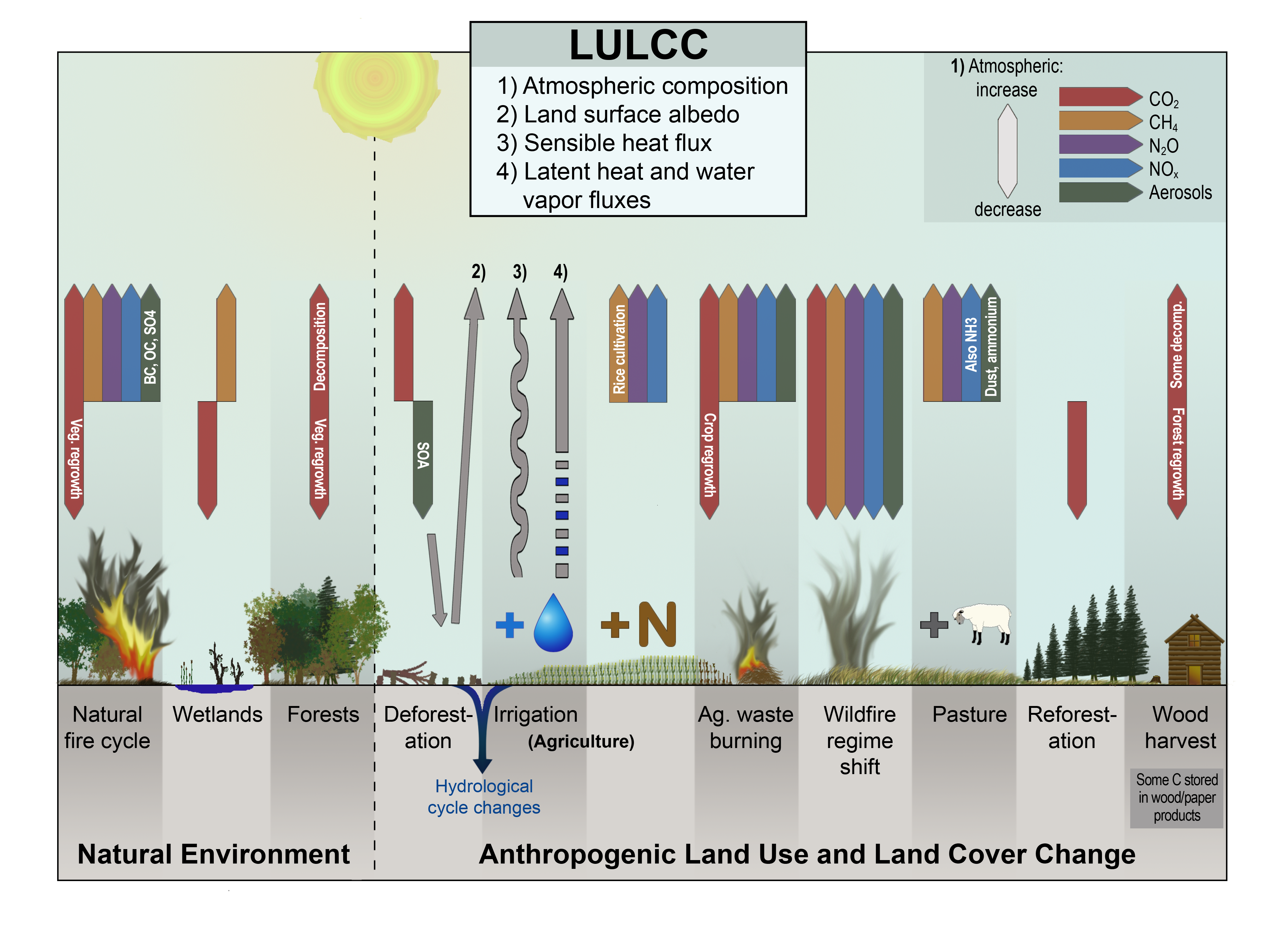
This graphical representation summarizes land–atmosphere interactions from natural and anthropogenic land-use and land-cover change (LULCC) contributions to radiative forcing. Emissions and sequestration of carbon and fluxes of nitrogen oxides, aerosols, and water shown here were used to calculate net radiative forcing from LULCC. (Figure source: Ward et al. 20145 ).
10.2: Terrestrial Ecosystem Interactions with the Climate System
Other chapters of this report discuss changes in temperature (Ch. 6: Temperature Change), precipitation (Ch. 7: Precipitation Change), hydrology (Ch. 8: Droughts, Floods, and Wildfires), and extreme events (Ch. 9: Extreme Storms). Collectively, these processes affect the phenology, structure, productivity, and biogeochemical processes of all terrestrial ecosystems, and as such, climate change will alter land cover and ecosystem services.
10.2.1 Land Cover and Climate Forcing
Changes in land cover and land use have long been recognized as important contributors to global climate forcing (e.g., Feddema et al. 20057 ). Historically, studies that account for the contribution of the land cover to radiative forcing have accounted for albedo forcings only and not those from changes in land surface geophysical properties (e.g., plant transpiration, evaporation from soils, plant community structure and function) or in aerosols. Physical climate effects from land-cover or land-use change do not lend themselves directly to quantification using the traditional radiative forcing concept. However, a framework to attribute the indirect contributions of land cover to radiative forcing and the climate system—including effects on seasonal and interannual soil moisture and latent/sensible heat, evapotranspiration, biogeochemical cycle (CO2) fluxes from soils and plants, aerosol and aerosol precursor emissions, ozone precursor emissions, and snowpack—was reported in NRC.8 Predicting future consequences of changes in land cover on the climate system will require not only the traditional calculations of surface albedo but also surface net radiation partitioning between latent and sensible heat exchange and the effects of resulting changes in biogeochemical trace gas and aerosol fluxes. Future trajectories of land use and land cover change are uncertain and will depend on population growth, changes in agricultural yield driven by the competing demands for production of fuel (i.e., bioenergy crops), food, feed, and fiber as well as urban expansion. The diversity of future land cover and land use changes as implemented by the models that developed the Representative Concentration Pathways (RCPs) to attain target goals of radiative forcing by 2100 is discussed by Hurtt et al.9 For example, the higher scenario (RCP8.5)10 features an increase of cultivated land by about 185 million hectares from 2000 to 2050 and another 120 million hectares from 2050 to 2100. In the mid-high scenario (RCP6.0)—the Asia Pacific Integrated Model (AIM),11 urban land use increases due to population and economic growth while cropland area expands due to increasing food demand. Grassland areas decline while total forested area extent remains constant throughout the century.9 The Global Change Assessment Model (GCAM), under a lower scenario (RCP4.5), preserved and expanded forested areas throughout the 21st century. Agricultural land declined slightly due to this afforestation, yet food demand is met through crop yield improvements, dietary shifts, production efficiency, and international trade.9 ,12 As with the higher scenario (RCP8.5), the even lower scenario (RCP2.6)13 reallocated agricultural production from developed to developing countries, with increased bioenergy production.9 Continued land-use change is projected across all RCPs (2.6, 4.5, 6.0, and 8.5) and is expected to contribute between 0.9 and 1.9 W/m2 to direct radiative forcing by 2100.5 The RCPs demonstrate that land-use management and change combined with policy, demographic, energy technological innovations and change, and lifestyle changes all contribute to future climate (see Ch. 4: Projections for more detail on RCPs).14
Traditional calculations of radiative forcing by land-cover change yield small forcing values (Ch. 2: Physical Drivers of Climate Change) because they account only for changes in surface albedo (e.g., Myhre and Myhre 2003;15 Betts et al. 2007;16 Jones et al. 201517 ). Recent assessments (Myhre et al. 20134 and references therein) are beginning to calculate the relative contributions of land-use and land-cover change (LULCC) to radiative forcing in addition to albedo and/or aerosols.5 Radiative forcing data reported in this chapter are largely from observations (see Table 8.2 in Myhre et al. 20134 ). Ward et al.5 performed an independent modeling study to partition radiative forcing from natural and anthropogenic land use and land cover change and related land management activities into contributions from carbon dioxide (CO2), methane (CH4), nitrous oxide (N2O), aerosols, halocarbons, and ozone (O3).
The more extended effects of land–atmosphere interactions from natural and anthropogenic land-use and land-cover change (LULCC; Figure 10.1) described above have recently been reviewed and estimated by atmospheric constituent (Figure 10.2).4 ,5 The combined albedo and greenhouse gas radiative forcing for land-cover change is estimated to account for 40% ± 16% of the human-caused global radiative forcing from 1850 to 2010 (Figure 10.2).5 These calculations for total radiative forcing (from LULCC sources and all other sources) are consistent with Myhre et al. 20134 (2.23 W/m2 and 2.22 W/m2 for Ward et al. 20145 and Myhre et al. 20134 , respectively). The contributions of CO2, CH4, N2O, and aerosols/O3/albedo effects to total LULCC radiative forcing are about 47%, 34%, 15%, and 4%, respectively, highlighting the importance of non-albedo contributions to LULCC and radiative forcing. The net radiative forcing due specifically to fire—after accounting for short-lived forcing agents (O3 and aerosols), long-lived greenhouse gases, and land albedo change both now and in the future—is estimated to be near zero due to regrowth of forests which offsets the release of CO2 from fire.18
10.2.2 Land Cover and Climate Feedbacks
Earth system models differ significantly in projections of terrestrial carbon uptake,19 with large uncertainties in the effects of increasing atmospheric CO2 concentrations (i.e., CO2 fertilization) and nutrient downregulation on plant productivity, as well as the strength of carbon cycle feedbacks (Ch. 2: Physical Drivers of Climate Change).20 ,21 When CO2 effects on photosynthesis and transpiration are removed from global gridded crop models, simulated response to climate across the models is comparable, suggesting that model parameterizations representing these processes remain uncertain.22
A recent analysis shows large-scale greening in the Arctic and boreal regions of North America and browning in the boreal forests of eastern Alaska for the period 1984–2012.23 Satellite observations and ecosystem models suggest that biogeochemical interactions of carbon dioxide (CO2) fertilization, nitrogen (N) deposition, and land-cover change are responsible for 25%–50% of the global greening of the Earth and 4% of Earth’s browning between 1982 and 2009.24 ,25 While several studies have documented significant increases in the rate of green-up periods, the lengthening of the growing season (Section 10.3.1) also alters the timing of green-up (onset of growth) and brown-down (senescence); however, where ecosystems become depleted of water resources as a result of a lengthening growing season, the actual period of productive growth can be truncated.26
Figure 10.2

Anthropogenic radiative forcing (RF) contributions, separated by land-use and land-cover change (LULCC) and non-LULCC sources (green and maroon bars, respectively), are decomposed by atmospheric constituent to year 2010 in this diagram, using the year 1850 as the reference. Total anthropogenic RF contributions by atmospheric constituent4
(see also Figure 2.3) are shown for comparison (yellow bars). Error bars represent uncertainties for total anthropogenic RF (yellow bars) and for the LULCC components (green bars).5 The SUM bars indicate the net RF when all anthropogenic forcing agents are combined. (Figure source: Ward et al. 20145 ).
Large-scale die-off and disturbances resulting from climate change have potential effects beyond the biogeochemical and carbon cycle effects. Biogeophysical feedbacks can strengthen or reduce climate forcing. The low albedo of boreal forests provides a positive feedback, but those albedo effects are mitigated in tropical forests through evaporative cooling; for temperate forests, the evaporative effects are less clear.27 Changes in surface albedo, evaporation, and surface roughness can have feedbacks to local temperatures that are larger than the feedback due to the change in carbon sequestration.28 Forest management frameworks (e.g., afforestation, deforestation, and avoided deforestation) that account for biophysical (e.g., land surface albedo and surface roughness) properties can be used as climate protection or mitigation strategies.29
10.2.3 Temperature Change
Interactions between temperature changes, land cover, and biogeochemistry are more complex than commonly assumed. Previous research suggested a fairly direct relationship between increasing temperatures, longer growing seasons (see Section 10.3.1), increasing plant productivity (e.g., Walsh et al. 201430 ), and therefore also an increase in CO2 uptake. Without water or nutrient limitations, increased CO2 concentrations and warm temperatures have been shown to extend the growing season, which may contribute to longer periods of plant activity and carbon uptake, but do not affect reproduction rates.31 However, a longer growing season can also increase plant water demand, affecting regional water availability, and result in conditions that exceed plant physiological thresholds for growth, producing subsequent feedbacks to radiative forcing and climate. These consequences could offset potential benefits of a longer growing season (e.g., Georgakakos et al. 201432 ; Hibbard et al. 201433 ). For instance, increased dry conditions can lead to wildfire (e.g., Hatfield et al. 2014;34 Joyce et al. 2014;35 Ch. 8: Droughts, Floods and Wildfires) and urban temperatures can contribute to urban-induced thunderstorms in the southeastern United States.36 Temperature benefits of early onset of plant development in a longer growing season can be offset by 1) freeze damage caused by late-season frosts; 2) limits to growth because of shortening of the photoperiod later in the season; or 3) by shorter chilling periods required for leaf unfolding by many plants.37 ,38 MODIS data provided insight into the coterminous U.S. 2012 drought, when a warm spring reduced the carbon cycle impact of the drought by inducing earlier carbon uptake.39 New evidence points to longer temperature-driven growing seasons for grasslands that may facilitate earlier onset of growth, but also that senescence is typically earlier.40 In addition to changing CO2 uptake, higher temperatures can also enhance soil decomposition rates, thereby adding more CO2 to the atmosphere. Similarly, temperature, as well as changes in the seasonality and intensity of precipitation, can influence nutrient and water availability, leading to both shortages and excesses, thereby influencing rates and magnitudes of decomposition.1
10.2.4 Water Cycle Changes
The global hydrological cycle is expected to intensify under climate change as a consequence of increased temperatures in the troposphere. The consequences of the increased water-holding capacity of a warmer atmosphere include longer and more frequent droughts and less frequent but more severe precipitation events and cyclonic activity (see Ch. 9: Extreme Storms for an in-depth discussion of extreme storms). More intense rain events and storms can lead to flooding and ecosystem disturbances, thereby altering ecosystem function and carbon cycle dynamics. For an extensive review of precipitation changes and droughts, floods, and wildfires, see Chapters 7 and 8 in this report, respectively.
From the perspective of the land biosphere, drought has strong effects on ecosystem productivity and carbon storage by reducing photosynthesis and increasing the risk of wildfire, pest infestation, and disease susceptibility. Thus, droughts of the future will affect carbon uptake and storage, leading to feedbacks to the climate system (Chapter 2, Section 2.6.2; also see Chapter 11 for Arctic/climate/wildfire feedbacks).41 Reduced productivity as a result of extreme drought events can also extend for several years post-drought (i.e., drought legacy effects).42 ,43 ,44 In 2011, the most severe drought on record in Texas led to statewide regional tree mortality of 6.2%, or nearly nine times greater than the average annual mortality in this region (approximately 0.7%).45 The net effect on carbon storage was estimated to be a redistribution of 24–30 TgC from the live to dead tree carbon pool, which is equal to 6%–7% of pre-drought live tree carbon storage in Texas state forestlands.45 Another way to think about this redistribution is that the single Texas drought event equals approximately 36% of annual global carbon losses due to deforestation and land-use change.46 The projected increases in temperatures and in the magnitude and frequency of heavy precipitation events, changes to snowpack, and changes in the subsequent water availability for agriculture and forestry may lead to similar rates of mortality or changes in land cover. Increasing frequency and intensity of drought across northern ecosystems reduces total observed organic matter export, has led to oxidized wetland soils, and releases stored contaminants into streams after rain events.47
10.2.5 Biogeochemistry
Terrestrial biogeochemical cycles play a key role in Earth’s climate system, including by affecting land–atmosphere fluxes of many aerosol precursors and greenhouse gases, including carbon dioxide (CO2), methane (CH4), and nitrous oxide (N2O). As such, changes in the terrestrial ecosphere can drive climate change. At the same time, biogeochemical cycles are sensitive to changes in climate and atmospheric composition.
Increased atmospheric CO2 concentrations are often assumed to lead to increased plant production (known as CO2 fertilization) and longer-term storage of carbon in biomass and soils. Whether increased atmospheric CO2 will continue to lead to long-term storage of carbon in terrestrial ecosystems depends on whether CO2 fertilization simply intensifies the rate of short-term carbon cycling (for example, by stimulating respiration, root exudation, and high turnover root growth), how water and other nutrients constrain CO2 fertilization, or whether the additional carbon is used by plants to build more wood or tissues that, once senesced, decompose into long-lived soil organic matter. Under increased CO2 concentrations, plants have been observed to optimize water use due to reduced stomatal conductance, thereby increasing water-use efficiency.48 This change in water-use efficiency can affect plants’ tolerance to stress and specifically to drought.49 Due to the complex interactions of the processes that govern terrestrial biogeochemical cycling, terrestrial ecosystem responses to increasing CO2 levels remain one of the largest uncertainties in long-term climate feedbacks and therefore in predicting longer-term climate change (Ch. 2: Physical Drivers of Climate Change).
Nitrogen is a principal nutrient for plant growth and can limit or stimulate plant productivity (and carbon uptake), depending on availability. As a result, increased nitrogen deposition and natural nitrogen-cycle responses to climate change will influence the global carbon cycle. For example, nitrogen limitation can inhibit the CO2 fertilization response of plants to elevated atmospheric CO2 (e.g., Norby et al. 2005;50 Zaehle et al. 201051 ). Conversely, increased decomposition of soil organic matter in response to climate warming increases nitrogen mineralization. This shift of nitrogen from soil to vegetation can increase ecosystem carbon storage.46 ,52 While the effects of increased nitrogen deposition may counteract some nitrogen limitation on CO2 fertilization, the importance of nitrogen in future carbon–climate interactions is not clear. Nitrogen dynamics are being integrated into the simulation of land carbon cycle modeling, but only two of the models in CMIP5 included coupled carbon–nitrogen interactions.53
Many factors, including climate, atmospheric CO2 concentrations, and nitrogen deposition rates influence the structure of the plant community and therefore the amount and biochemical quality of inputs into soils.54 ,55 ,56 For example, though CO2 losses from soils may decrease with greater nitrogen deposition, increased emissions of other greenhouse gases, such as methane (CH4) and nitrous oxide (N2O), can offset the reduction in CO2.57 The dynamics of soil organic carbon under the influence of climate change is poorly understood and therefore not well represented in models. As a result, there is high uncertainty in soil carbon stocks in model simulations.58 ,59
Future emissions of many aerosol precursors are expected to be affected by a number of climate-related factors, in part because of changes in aerosol and aerosol precursors from the terrestrial biosphere. For example, volatile organic compounds (VOCs) are a significant source of secondary organic aerosols, and biogenic sources of VOCs exceed emissions from the industrial and transportation sectors.60 Isoprene is one of the most important biogenic VOCs, and isoprene emissions are strongly dependent on temperature and light, as well as other factors like plant type and leaf age.60 Higher temperatures are expected to lead to an increase in biogenic VOC emissions. Atmospheric CO2 concentration can also affect isoprene emissions (e.g., Rosenstiel et al. 200361 ). Changes in biogenic VOC emissions can impact aerosol formation and feedbacks with climate (Ch. 2: Physical Drivers of Climate Change, Section 2.6.1; Feedbacks via changes in atmospheric composition). Increased biogenic VOC emissions can also impact ozone and the atmospheric oxidizing capacity.62 Conversely, increases in nitrogen oxide (NOx) pollution produce tropospheric ozone (O3), which has damaging effects on vegetation. For example, a recent study estimated yield losses for maize and soybean production of up to 5% to 10% due to increases in O3.63
10.2.6 Extreme Events and Disturbance
This section builds on the physical overview provided in earlier chapters to frame how the intersections of climate, extreme events, and disturbance affect regional land cover and biogeochemistry. In addition to overall trends in temperature (Ch. 6: Temperature Change) and precipitation (Ch. 7: Precipitation Change), changes in modes of variability such as the Pacific Decadal Oscillation (PDO) and the El Niño–Southern Oscillation (ENSO) (Ch. 5: Circulation and Variability) can contribute to drought in the United States, which leads to unanticipated changes in disturbance regimes in the terrestrial biosphere (e.g., Kam et al. 201464 ). Extreme climatic events can increase the susceptibility of ecosystems to invasive plants and plant pests by promoting transport of propagules into affected regions, decreasing the resistance of native communities to establishment, and by putting existing native species at a competitive disadvantage.65 For example, drought may exacerbate the rate of plant invasions by non-native species in rangelands and grasslands.45 Land-cover changes such as encroachment and invasion of non-native species can in turn lead to increased frequency of disturbance such as fire. Disturbance events alter soil moisture, which, in addition to being affected by evapotranspiration and precipitation (Ch. 8: Droughts, Floods, and Wildfires), is controlled by canopy and rooting architecture as well as soil physics. Invasive plants may be directly responsible for changes in fire regimes through increased biomass, changes in the distribution of flammable biomass, increased flammability, and altered timing of fuel drying, while others may be “fire followers” whose abundances increase as a result of shortening the fire return interval (e.g., Lambert et al. 201066 ). Changes in land cover resulting from alteration of fire return intervals, fire severity, and historical disturbance regimes affect long-term carbon exchange between the atmosphere and biosphere (e.g., Moore et al. 201645 ). Recent extensive diebacks and changes in plant cover due to drought have interacted with regional carbon cycle dynamics, including carbon release from biomass and reductions in carbon uptake from the atmosphere; however, plant regrowth may offset emissions.67 The 2011–2015 meteorological drought in California (described in Ch. 8: Droughts, Floods, and Wildfires), combined with future warming, will lead to long-term changes in land cover, leading to increased probability of climate feedbacks (e.g., drought and wildfire) and in ecosystem shifts.68 California’s recent drought has also resulted in measureable canopy water losses, posing long-term hazards to forest health and biophysical feedbacks to regional climate.44 ,69 ,70 Multiyear or severe meteorological and hydrological droughts (see Ch. 8: Droughts, Floods, and Wildfires for definitions) can also affect stream biogeochemistry and riparian ecosystems by concentrating sediments and nutrients.67
Changes in the variability of hurricanes and winter storm events (Ch. 9: Extreme Storms) also affect the terrestrial biosphere, as shown in studies comparing historic and future (projected) extreme events in the western United States and how these translate into changes in regional water balance, fire, and streamflow. Composited across 10 global climate models (GCMs), summer (June–August) water-balance deficit in the future (2030–2059) increases compared to that under historical (1916–2006) conditions. Portions of the Southwest that have significant monsoon precipitation and some mountainous areas of the Pacific Northwest are exempt from this deficit.71 Projections for 2030–2059 suggest that extremely low flows that have historically occurred (1916–2006) in the Columbia Basin, upper Snake River, southeastern California, and southwestern Oregon are less likely to occur. Given the historical relationships between fire occurrence and drought indicators such as water-balance deficit and streamflow, climate change can be expected to have significant effects on fire occurrence and area burned.71 ,72 ,73
Climate change in the northern high latitudes is directly contributing to increased fire occurrence (Ch. 11: Arctic Changes); in the coterminous United States, climate-induced changes in fires, changes in direct human ignitions, and land-management practices all significantly contribute to wildfire trends. Wildfires in the western United States are often ignited by lightning, but management practices such as fire suppression contribute to fuels and amplify the intensity and spread of wildfire. Fires initiated from unintentional ignition, such as by campfires, or intentional human-caused ignitions are also intensified by increasingly dry and vulnerable fuels, which build up with fire suppression or human settlements (See also Ch. 8: Droughts, Floods, and Wildfires).
10.3: Climate Indicators and Agricultural and Forest Responses
Recent studies indicate a correlation between the expansion of agriculture and the global amplitude of CO2 uptake and emissions.74 ,75 Conversely, agricultural production is increasingly disrupted by climate and extreme weather events, and these effects are expected to be augmented by mid-century and beyond for most crops.76 ,77 Precipitation extremes put pressure on agricultural soil and water assets and lead to increased irrigation, shrinking aquifers, and ground subsidence.
10.3.1 Changes in the Frost-Free and Growing Seasons
The concept that longer growing seasons are increasing productivity in some agricultural and forested ecosystems was discussed in the Third National Climate Assessment (NCA3).6 However, there are other consequences to a lengthened growing season that can offset gains in productivity. Here we discuss these emerging complexities as well as other aspects of how climate change is altering and interacting with terrestrial ecosystems. The growing season is the part of the year in which temperatures are favorable for plant growth. A basic metric by which this is measured is the frost-free period. The U.S. Department of Agriculture Natural Resources Conservation Service defines the frost-free period using a range of thresholds. They calculate the average date of the last day with temperature below 24°F (−4.4°C), 28°F (−2.2°C), and 32°F (0°C) in the spring and the average date of the first day with temperature below 24°F, 28°F, and 32°F in the fall, at various probabilities. They then define the frost-free period at three index temperatures (32°F, 28°F, and 24°F), also with a range of probabilities. A single temperature threshold (for example, temperature below 32°F) is often used when discussing growing season; however, different plant cover-types (e.g., forest, agricultural, shrub, and tundra) have different temperature thresholds for growth, and different requirements/thresholds for chilling.34 ,78 For the purposes of this report, we use the metric with a 32°F (0°C) threshold to define the change in the number of “frost-free” days, and a temperature threshold of 41°F (5°C) as a first-order measure of how the growing season length has changed over the observational record.78
Figure 10.3
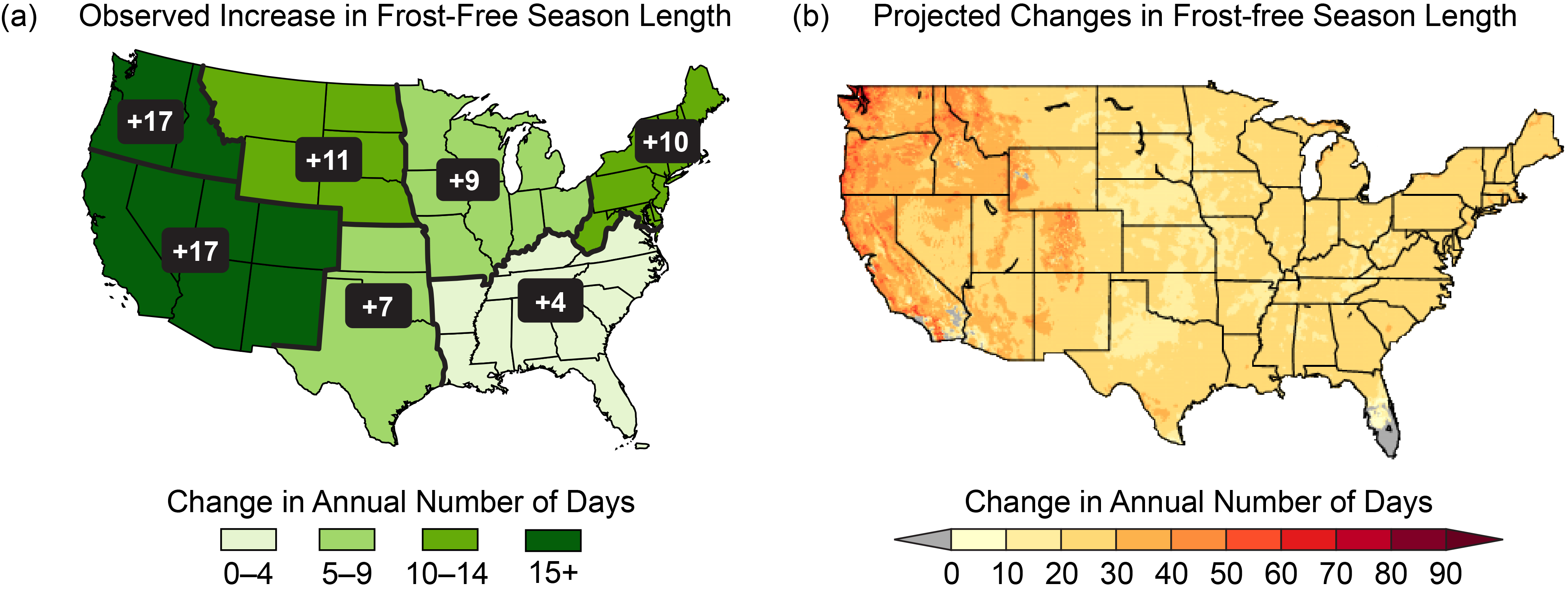
(a) Observed changes in the length of the frost-free season by region, where the frost-free season is defined as the number of days between the last spring occurrence and the first fall occurrence of a minimum temperature at or below 32°F. This change is expressed as the change in the average number of frost-free days in 1986–2015 compared to 1901–1960. (b) Projected changes in the length of the frost-free season at mid-century (2036–2065 as compared to 1976–2005) under the higher scenario (RCP8.5). Gray indicates areas that are not projected to experience a freeze in more than 10 of the 30 years (Figure source: (a) updated from Walsh et al. 2014;30 (b) NOAA NCEI and CICS-NC, data source: LOCA dataset).
The NCA3 reported an increase in the growing season length of as much as several weeks as a result of higher temperatures occurring earlier and later in the year (e.g., Walsh et al. 2014;30 Hatfield et al. 2014;34 Joyce et al. 201435 ). NCA3 used a threshold of 32°F (0°C) (i.e., the frost-free period) to define the growing season. An update to this finding is presented in Figures 10.3 and 10.4, which show changes in the frost-free period and growing season, respectively, as defined above. Overall, the length of the frost-free period has increased in the contiguous United States during the past century (Figure 10.3). However, growing season changes are more variable: growing season length increased until the late 1930s, declined slightly until the early 1970s, increased again until about 1990, and remained quasi-stable thereafter (Figure 10.4). This contrasts somewhat with changes in the length of the frost-free period presented in NCA3, which showed a continuing increase after 1980. This difference is attributable to the temperature thresholds used in each indicator to define the start and end of these periods. Specifically, there are now more frost-free days (32°F threshold) in winter than the growing season (41°F threshold).
Figure 10.4
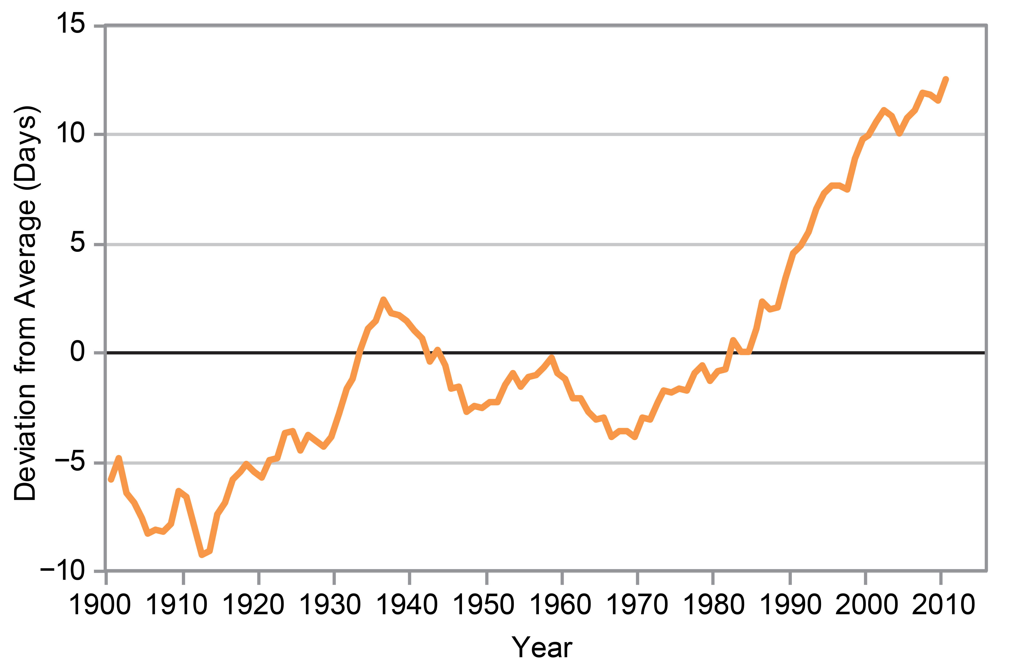
The length of the growing season in the contiguous 48 states compared with a long-term average (1895–2015), where “growing season” is defined by a daily minimum temperature threshold of 41°F. For each year, the line represents the number of days shorter or longer than the long-term average. The line was smoothed using an 11-year moving average. Choosing a different long-term average for comparison would not change the shape of the data over time. (Figure source: Kunkel 20162 ).
The lengthening of the growing season has been somewhat greater in the northern and western United States, which experienced increases of 1–2 weeks in many locations. In contrast, some areas in the Midwest, Southern Great Plains, and the Southeast had decreases of a week or more between the periods 1986–2015 and 1901–1960.2 These differences reflect the more general pattern of warming and cooling nationwide (Ch. 6: Temperature Changes). Observations and models have verified that the growing season has generally increased plant productivity over most of the United States.25
Consistent with increases in growing season length and the coldest temperature of the year, plant hardiness zones have shifted northward in many areas.79 The widespread increase in temperature has also impacted the distribution of other climate zones in parts of the United States. For instance, there have been moderate changes in the range of the temperate and continental climate zones of the eastern United States since 195080 as well as changes in the coverage of some extreme climate zones in the western United States. In particular, the spatial extent of the “alpine tundra” zone has decreased in high-elevation areas,81 while the extent of the “hot arid” zone has increased in the Southwest.82
The period over which plants are actually productive, that is, their true growing season, is a function of multiple climate factors, including air temperature, number of frost-free days, and rainfall, as well as biophysical factors, including soil physics, daylight hours, and the biogeochemistry of ecosystems.83 Temperature-induced changes in plant phenology, like flowering or spring leaf onset, could result in a timing mismatch (phenological asynchrony) with pollinator activity, affecting seasonal plant growth and reproduction and pollinator survival.84 ,85 ,86 ,87 Further, while growing season length is generally referred to in the context of agricultural productivity, the factors that govern which plant types will grow in a given location are common to all plants whether they are in agricultural, natural, or managed landscapes. Changes in both the length and the seasonality of the growing season, in concert with local environmental conditions, can have multiple effects on agricultural productivity and land cover.
In the context of agriculture, a longer growing season could allow for the diversification of cropping systems or allow multiple harvests within a growing season. For example, shifts in cold hardiness zones across the contiguous United States suggest widespread expansion of thermally suitable areas for the cultivation of cold-intolerant perennial crops88 as well as for biological invasion of non-native plants and plant pests.89 However, changes in available water, conversion from dry to irrigated farming, and changes in sensible and latent heat exchange associated with these shifts need to be considered. Increasingly dry conditions under a longer growing season can alter terrestrial organic matter export and catalyze oxidation of wetland soils, releasing stored contaminants (for example, copper and nickel) into streamflow after rainfall.47 Similarly, a longer growing season, particularly in years where water is limited, is not due to warming alone, but is exacerbated by higher atmospheric CO2 concentrations that extend the active period of growth by plants.31 Longer growing seasons can also limit the types of crops that can be grown, encourage invasive species encroachment or weed growth, or increase demand for irrigation, possibly beyond the limits of water availability. They could also disrupt the function and structure of a region’s ecosystems and could, for example, alter the range and types of animal species in the area.
A longer and temporally shifted growing season also affects the role of terrestrial ecosystems in the carbon cycle. Neither seasonality of growing season (spring and summer) nor carbon, water, and energy fluxes should be interpreted separately when analyzing the impacts of climate extremes such as drought (Ch. 8: Droughts, Floods, and Wildfires).39 ,90 Observations and data-driven model studies suggest that losses in net terrestrial carbon uptake during record warm springs followed by severely hot and dry summers can be largely offset by carbon gains in record-exceeding warmth and early arrival of spring.39 Depending on soil physics and land cover, a cool spring, however, can deplete soil water resources less rapidly, making the subsequent impacts of precipitation deficits less severe.90 Depletion of soil moisture through early plant activity in a warm spring can potentially amplify summer heating, a typical lagged direct effect of an extremely warm spring.42 Ecosystem responses to the phenological changes of timing and extent of growing season and subsequent biophysical feedbacks are therefore strongly dependent on the timing of climate extremes (Ch. 8: Droughts, Floods, and Wildfires; Ch. 9: Extreme Storms).90
The global Coupled Model Intercomparison Project Phase 5 (CMIP5) analyses did not explicitly explore future changes to the growing season length. Many of the projected changes in North American climate are generally consistent across CMIP5 models, but there is substantial inter-model disagreement in projections of some metrics important to productivity in biophysical systems, including the sign of regional precipitation changes and extreme heat events across the northern United States.91
10.3.2 Water Availability and Drought
Drought is generally parameterized in most agricultural models as limited water availability and is an integrated response of both meteorological and agricultural drought, as described in Chapter 8: Droughts, Floods, and Wildfires. However, physiological as well as biophysical processes that influence land cover and biogeochemistry interact with drought through stomatal closure induced by elevated atmospheric CO2 levels.48 ,49 This has direct impacts on plant transpiration, atmospheric latent heat fluxes, and soil moisture, thereby influencing local and regional climate. Drought is often offset by management through groundwater withdrawals, with increasing pressure on these resources to maintain plant productivity. This results in indirect climate effects by altering land surface exchange of water and energy with the atmosphere.92
10.3.3 Forestry Considerations
Climate change and land-cover change in forested areas interact in many ways, such as through changes in mortality rates driven by changes in the frequency and magnitude of fire, insect infestations, and disease. In addition to the direct economic benefits of forestry, unquantified societal benefits include ecosystem services, like protection of watersheds and wildlife habitat, and recreation and human health value. United States forests and related wood products also absorb and store the equivalent of 16% of all CO2 emitted by fossil fuel burning in the United States each year.6 Climate change is expected to reduce the carbon sink strength of forests overall.
Effective management of forests offers the opportunity to reduce future climate change—for example, as given in proposals for Reduced Emissions from Deforestation and forest Degradation (REDD+; https://www.forestcarbonpartnership.org/what-redd) in developing countries and tropical ecosystems (see Ch. 14: Mitigation)—by capturing and storing carbon in forest ecosystems and long-term wood products.93 Afforestation in the United States has the potential to capture and store 225 million tons of additional carbon per year from 2010 to 2110.94 ,95 However, the projected maturation of United States forests96 and land-cover change, driven in particular by the expansion of urban and suburban areas along with projected increased demands for food and bioenergy, threaten the extent of forests and their carbon storage potential.97
Changes in growing season length, combined with drought and accompanying wildfire are reshaping California’s mountain ecosystems. The California drought led to the lowest snowpack in 500 years, the largest wildfires in post-settlement history, greater than 23% stress mortality in Sierra mid-elevation forests, and associated post-fire erosion.69 It is anticipated that slow recovery, possibly to different ecosystem types, with numerous shifts to species’ ranges will result in long-term changes to land surface biophysical as well as ecosystem structure and function in this region (http://www.fire.ca.gov/treetaskforce/).69
While changes in forest stocks, composition, and the ultimate use of forest products can influence net emissions and climate, the future net changes in forest stocks remain uncertain.9 ,27 ,98 ,99 ,100 This uncertainty is due to a combination of uncertainties in future population size, population distribution and subsequent land-use change, harvest trends, wildfire management practices (for example, large-scale thinning of forests), and the impact of maturing U.S. forests.
10.4: Urban Environments and Climate Change
Urban areas exhibit several characteristics that affect land-surface and geophysical attributes, including building infrastructure (rougher, more uneven surfaces compared to rural or natural systems), increased emissions and concentrations of aerosols and other greenhouse gasses, and increased anthropogenic heat sources.101 ,102 The understanding that urban areas modify their surrounding environment has been accepted for over a century, but the mechanisms through which this occurs have only begun to be understood and analyzed for more than 40 years.102 ,103 Prior to the 1970s, the majority of urban climate research was observational and descriptive,104 but since that time, more importance has been given to physical dynamics that are a function of land surface (for example, built environment and change to surface roughness); hydrologic, aerosol, and other greenhouse gas emissions; thermal properties of the built environment; and heat generated from human activities (Seto et al. 2016105 and references therein).
There is now strong evidence that urban environments modify local microclimates, with implications for regional and global climate change.102 ,104 Urban systems affect various climate attributes, including temperature, rainfall intensity and frequency, winter precipitation (snowfall), and flooding. New observational capabilities—including NASA’s dual polarimetric radar, advanced satellite remote sensing (for example, the Global Precipitation Measurement Mission-GPM), and regionalized, coupled land–surface–atmospheric modeling systems for urban systems—are now available to evaluate aspects of daytime and nighttime temperature fluctuations; urban precipitation; contribution of aerosols; how the urban built environment impacts the seasonality and type of precipitation (rain or snow) as well as the amount and distribution of precipitation; and the significance of the extent of urban metropolitan areas.101 ,102 ,106 ,107
The urban heat island (UHI) is characterized by increased surface and canopy temperatures as a result of heat-retaining asphalt and concrete, a lack of vegetation, and anthropogenic generation of heat and greenhouse gasses.107 The heat gain due to the storage capacity of urban built structures, reductions in local evapotranspiration, and anthropogenically generated heat alter the spatio-temporal pattern of temperature and leads to the UHI phenomenon. The UHI physical processes that affect the climate system include generation of heat storage in buildings during the day, nighttime release of latent heat storage by buildings, and sensible heat generated by human activities, include heating of buildings, air conditioning, and traffic.108
The strength of the effect is correlated with the spatial extent and population density of urban areas; however, because of varying definitions of urban vs. non-urban, impervious surface area is a more objective metric for estimating the extent and intensity of urbanization.109 Based on land surface temperature measurements, on average, the UHI effect increases urban temperature by 5.2°F (2.9°C), but it has been measured at 14.4°F (8°C) in cities built in areas dominated by temperate forests.109 In arid regions, however, urban areas can be more than 3.6°F (2°C) cooler than surrounding shrublands.110 Similarly, urban settings lose up to 12% of precipitation through impervious surface runoff, versus just over 3% loss to runoff in vegetated regions. Carbon losses from the biosphere to the atmosphere through urbanization account for almost 2% of the continental terrestrial biosphere total, a significant proportion given that urban areas only account for around 1% of land in the United States.110 Similarly, statistical analyses of the relationship between climate and urban land use suggest an empirical relationship between the patterns of urbanization and precipitation deficits during the dry season. Causal factors for this reduction may include changes to runoff (for example, impervious-surface versus natural-surface hydrology) that extend beyond the urban heat island effect and energy-related aerosol emissions.111
The urban heat island effect is more significant during the night and during winter than during the day, and it is affected by the shape, size, and geometry of buildings in urban centers as well as by infrastructure along gradients from urban to rural settlements.101 ,105 ,106 Recent research points to mounting evidence that urbanization also affects cycling of water, carbon, aerosols, and nitrogen in the climate system.106
Coordinated modeling and observational studies have revealed other mechanisms by which the physical properties of urban areas can influence local weather and climate. It has been suggested that urban-induced wind convergence can determine storm initiation; aerosol concentrations and composition then influence the amount of cloud water and ice present in the clouds. Aerosols can also influence updraft and downdraft intensities, their life span, and surface precipitation totals.107 A pair of studies investigated rainfall efficiency in sea-breeze thunderstorms and found that integrated moisture convergence in urban areas influenced storm initiation and mid-level moisture, thereby affecting precipitation dynamics.112 ,113
According to the World Bank, over 81% of the United States population currently resides in urban settings.114 Climate mitigation efforts to offset UHI are often stalled by the lack of quantitative data and understanding of the specific factors of urban systems that contribute to UHI. A recent study set out to quantitatively determine contributors to the intensity of UHI across North America.115 The study found that population strongly influenced nighttime UHI, but that daytime UHI varied spatially following precipitation gradients. The model applied in this study indicated that the spatial variation in the UHI signal was controlled most strongly by impacts on the atmospheric convection efficiency. Because of the impracticality of managing convection efficiency, results from Zhao et al.115 support albedo management as an efficient strategy to mitigate UHI on a large scale.
References
- Adams, H. D., A. D. Collins, S. P. Briggs, M. Vennetier, L. T. Dickman, S. A. Sevanto, N. Garcia-Forner, H. H. Powers, and N. G. McDowell, 2015: Experimental drought and heat can delay phenological development and reduce foliar and shoot growth in semiarid trees. Global Change Biology, 21, 4210–4220, doi:10.1111/gcb.13030. ↩
- Anav, A., P. Friedlingstein, M. Kidston, L. Bopp, P. Ciais, P. Cox, C. Jones, M. Jung, R. Myneni, and Z. Zhu, 2013: Evaluating the land and ocean components of the global carbon cycle in the CMIP5 earth system models. Journal of Climate, 26, 6801–6843, doi:10.1175/jcli-d-12-00417.1. ↩
- Anderegg, W. R. L., C. Schwalm, F. Biondi, J. J. Camarero, G. Koch, M. Litvak, K. Ogle, J. D. Shaw, E. Shevliakova, A. P. Williams, A. Wolf, E. Ziaco, and S. Pacala, 2015: Pervasive drought legacies in forest ecosystems and their implications for carbon cycle models. Science, 349, 528–532, doi:10.1126/science.aab1833. ↩
- Anderson, R. G., J. G. Canadell, J. T. Randerson, R. B. Jackson, B. A. Hungate, D. D. Baldocchi, G. A. Ban-Weiss, G. B. Bonan, K. Caldeira, L. Cao, N. S. Diffenbaugh, K. R. Gurney, L. M. Kueppers, B. E. Law, S. Luyssaert, and T. L. O’Halloran, 2011: Biophysical considerations in forestry for climate protection. Frontiers in Ecology and the Environment, 9, 174–182, doi:10.1890/090179. ↩
- Ashley, W. S., M. L. Bentley, and J. A. Stallins, 2012: Urban-induced thunderstorm modification in the Southeast United States. Climatic Change, 113, 481–498, doi:10.1007/s10584-011-0324-1. ↩
- Asner, G. P., P. G. Brodrick, C. B. Anderson, N. Vaughn, D. E. Knapp, and R. E. Martin, 2016: Progressive forest canopy water loss during the 2012–2015 California drought. Proceedings of the National Academy of Sciences, 113, E249–E255, doi:10.1073/pnas.1523397113. ↩
- Bank, W., 2017: Urban population (% of total): United States (1960-2015). World Bank Open Data. URL ↩
- Betts, R. A., P. D. Falloon, K. K. Goldewijk, and N. Ramankutty, 2007: Biogeophysical effects of land use on climate: Model simulations of radiative forcing and large-scale temperature change. Agricultural and Forest Meteorology, 142, 216–233, doi:10.1016/j.agrformet.2006.08.021. ↩
- Bonan, G. B., 2008: Forests and Climate Change: Forcings, Feedbacks, and the Climate Benefits of Forests. Science, 320, 1444–1449, doi:10.1126/science.1155121. ↩
- Bounoua, L., P. Zhang, G. Mostovoy, K. Thome, J. Masek, M. Imhoff, M. Shepherd, D. Quattrochi, J. Santanello, J. Silva, R. Wolfe, and A. M. Toure, 2015: Impact of urbanization on US surface climate. Environmental Research Letters, 10, 084010, doi:10.1088/1748-9326/10/8/084010. ↩
- Brown, D. G., C. Polsky, P. Bolstad, S. D. Brody, D. Hulse, R. Kroh, T. R. Loveland, and A. Thomson, 2014: Ch. 13: Land Use and Land Cover Change. J.M. Melillo, Terese (T.C.) Richmond, and G.W. Yohe, Eds., U.S. Global Change Research Program, 318–332. ↩
- Challinor, A. J., J. Watson, D. B. Lobell, S. M. Howden, D. R. Smith, and N. Chhetri, 2014: A meta-analysis of crop yield under climate change and adaptation. Nature Climate Change, 4, 287–291, doi:10.1038/nclimate2153. ↩
- Chan, D., and Q. Wu, 2015: Significant anthropogenic-induced changes of climate classes since 1950. Scientific Reports, 5, 13487, doi:10.1038/srep13487. ↩
- Ciais, P., C. Sabine, G. Bala, L. Bopp, V. Brovkin, J. Canadell, A. Chhabra, R. DeFries, J. Galloway, M. Heimann, C. Jones, C. Le Quéré, R. B. Myneni, S. Piao, and P. Thornton, 2013: Carbon and other biogeochemical cycles. T.F. Stocker, D. Qin, G.-K. Plattner, M. Tignor, S.K. Allen, J. Boschung, A. Nauels, Y. Xia, V. Bex, and P.M. Midgley, Eds., Cambridge University Press, 465–570. URL ↩
- Daly, C., M. P. Widrlechner, M. D. Halbleib, J. I. Smith, and W. P. Gibson, 2012: Development of a new USDA plant hardiness zone map for the United States. Journal of Applied Meteorology and Climatology, 51, 242–264, doi:10.1175/2010JAMC2536.1. ↩
- Diaz, H. F., and J. K. Eischeid, 2007: Disappearing “alpine tundra” Köppen climatic type in the western United States. Geophysical Research Letters, 34, L18707, doi:10.1029/2007GL031253. ↩
- Diez, J. M., C. M. D’Antonio, J. S. Dukes, E. D. Grosholz, J. D. Olden, C. J. B. Sorte, D. M. Blumenthal, B. A. Bradley, R. Early, I. Ibáñez, S. J. Jones, J. J. Lawler, and L. P. Miller, 2012: Will extreme climatic events facilitate biological invasions? Frontiers in Ecology and the Environment, 10, 249–257, doi:10.1890/110137. ↩
- Diffenbaugh, N. S., D. L. Swain, and D. Touma, 2015: Anthropogenic warming has increased drought risk in California. Proceedings of the National Academy of Sciences, 112, 3931–3936, doi:10.1073/pnas.1422385112. ↩
- EPA, 2005: Greenhouse Gas Mitigation Potential in U.S. Forestry and Agriculture. EPA 430-R-05-006. ↩
- EPA, 2016: Climate Change Indicators in the United States, 2016. 4th edition. 96 pp., U.S. Environmental Protection Agency. URL ↩
- Elsner, M. M., L. Cuo, N. Voisin, J. S. Deems, A. F. Hamlet, J. A. Vano, K. E. B. Mickelson, S. Y. Lee, and D. P. Lettenmaier, 2010: Implications of 21st century climate change for the hydrology of Washington State. Climatic Change, 102, 225–260, doi:10.1007/s10584-010-9855-0. ↩
- Feddema, J. J., K. W. Oleson, G. B. Bonan, L. O. Mearns, L. E. Buja, G. A. Meehl, and W. M. Washington, 2005: The importance of land-cover change in simulating future climates. Science, 310, 1674–1678, doi:10.1126/science.1118160. ↩
- Forrest, J. R. K., 2015: Plant–pollinator interactions and phenological change: What can we learn about climate impacts from experiments and observations? Oikos, 124, 4–13, doi:10.1111/oik.01386. ↩
- Frank, D. et al., 2015: Effects of climate extremes on the terrestrial carbon cycle: Concepts, processes and potential future impacts. Global Change Biology, 21, 2861–2880, doi:10.1111/gcb.12916. ↩
- Fridley, J. D., J. S. Lynn, J. P. Grime, and A. P. Askew, 2016: Longer growing seasons shift grassland vegetation towards more-productive species. Nature Climate Change, 6, 865–868, doi:10.1038/nclimate3032. ↩
- Fu, Y. H., H. Zhao, S. Piao, M. Peaucelle, S. Peng, G. Zhou, P. Ciais, M. Huang, A. Menzel, J. Penuelas, Y. Song, Y. Vitasse, Z. Zeng, and I. A. Janssens, 2015: Declining global warming effects on the phenology of spring leaf unfolding. Nature, 526, 104–107, doi:10.1038/nature15402. ↩
- Fujimori, S., T. Masui, and Y. Matsuoka, 2014: Development of a global computable general equilibrium model coupled with detailed energy end-use technology. Applied Energy, 128, 296–306, doi:10.1016/j.apenergy.2014.04.074. ↩
- G. Myhre, D. Shindell, F.-M. Bréon, W. Collins, J. Fuglestvedt, J. Huang, D. Koch, J.-F. Lamarque, D. Lee, B. Mendoza, T. Nakajima, A. Robock, G. Stephens, T. Takemura, and H. Zhang, 2013: Anthropogenic and natural radiative forcing. T.F. Stocker, D. Qin, G.-K. Plattner, M. Tignor, S.K. Allen, J. Boschung, A. Nauels, Y. Xia, V. Bex, and P.M. Midgley, Eds., Cambridge University Press, 659–740. URL ↩
- Galloway, J. N., W. H. Schlesinger, C. M. Clark, N. B. Grimm, R. B. Jackson, B. E. Law, P. E. Thornton, A. R. Townsend, and R. Martin, 2014: Ch. 15: Biogeochemical Cycles. J.M. Melillo, Terese (T.C.) Richmond, and G.W. Yohe, Eds., U.S. Global Change Research Program, 350–368. ↩
- Georgakakos, A., P. Fleming, M. Dettinger, C. Peters-Lidard, Terese (T.C.) Richmond, K. Reckhow, K. White, and D. Yates, 2014: Ch. 3: Water Resources. J.M. Melillo, T. (T. C.. Richmond, and G.W. Yohe, Eds., U.S. Global Change Research Program, 69–112. ↩
- Gray, J. M., S. Frolking, E. A. Kort, D. K. Ray, C. J. Kucharik, N. Ramankutty, and M. A. Friedl, 2014: Direct human influence on atmospheric CO2 seasonality from increased cropland productivity. Nature, 515, 398–401, doi:10.1038/nature13957. ↩
- Grimmond, C. S. B., H. C. Ward, and S. Kotthaus, 2016: Effects of urbanization on local and regional climate. K. C. Seto, W. D. Solecki, and C. A. Griffith, Eds., Routledge, 169–187. ↩
- Grundstein, A., 2008: Assessing climate change in the contiguous United States using a modified Thornthwaite climate classification scheme. The Professional Geographer, 60, 398–412, doi:10.1080/00330120802046695. ↩
- Gu, L., P. J. Hanson, W. Mac Post, D. P. Kaiser, B. Yang, R. Nemani, S. G. Pallardy, and T. Meyers, 2008: The 2007 eastern US spring freezes: Increased cold damage in a warming world? BioScience, 58, 253–262, doi:10.1641/b580311. ↩
- Guenther, A., T. Karl, P. Harley, C. Wiedinmyer, P. I. Palmer, and C. Geron, 2006: Estimates of global terrestrial isoprene emissions using MEGAN (Model of Emissions of Gases and Aerosols from Nature). Atmospheric Chemistry and Physics, 6, 3181–3210, doi:10.5194/acp-6-3181-2006. ↩
- Hansen, M. C., P. V. Potapov, R. Moore, M. Hancher, S. A. Turubanova, A. Tyukavina, D. Thau, S. V. Stehman, S. J. Goetz, T. R. Loveland, A. Kommareddy, A. Egorov, L. Chini, C. O. Justice, and J. R. G. Townshend, 2013: High-resolution global maps of 21st-century forest cover change. Science, 342, 850–853, doi:10.1126/science.1244693. ↩
- Hatfield, J., G. Takle, R. Grotjahn, P. Holden, R. C. Izaurralde, T. Mader, E. Marshall, and D. Liverman, 2014: Ch. 6: Agriculture. J.M. Melillo, Terese (T.C.) Richmond, and G.W. Yohe, Eds., U.S. Global Change Research Program, 150–174. ↩
- Hellmann, J. J., J. E. Byers, B. G. Bierwagen, and J. S. Dukes, 2008: Five potential consequences of climate change for invasive species. Conservation Biology, 22, 534–543, doi:10.1111/j.1523-1739.2008.00951.x. ↩
- Hibbard, K., T. Wilson, K. Averyt, R. Harriss, R. Newmark, S. Rose, E. Shevliakova, and V. Tidwell, 2014: Ch. 10: Energy, Water, and Land Use. J.M. Melillo, Terese (T.C.) Richmond, and G.W. Yohe, Eds., U.S. Global Change Research Program, 257–281. ↩
- Hidalgo, J., V. Masson, A. Baklanov, G. Pigeon, and L. Gimeno, 2008: Advances in urban cimate mdeling. Annals of the New York Academy of Sciences, 1146, 354–374, doi:10.1196/annals.1446.015. ↩
- Hoffman, F. M., J. T. Randerson, V. K. Arora, Q. Bao, P. Cadule, D. Ji, C. D. Jones, M. Kawamiya, S. Khatiwala, K. Lindsay, A. Obata, E. Shevliakova, K. D. Six, J. F. Tjiputra, E. M. Volodin, and T. Wu, 2014: Causes and implications of persistent atmospheric carbon dioxide biases in Earth System Models. Journal of Geophysical Research Biogeosciences, 119, 141–162, doi:10.1002/2013JG002381. ↩
- Hurtt, G. C. et al., 2011: Harmonization of land-use scenarios for the period 1500–2100: 600 years of global gridded annual land-use transitions, wood harvest, and resulting secondary lands. Climatic Change, 109, 117, doi:10.1007/s10584-011-0153-2. ↩
- Imhoff, M. L., P. Zhang, R. E. Wolfe, and L. Bounoua, 2010: Remote sensing of the urban heat island effect across biomes in the continental USA. Remote Sensing of Environment, 114, 504–513, doi:10.1016/j.rse.2009.10.008. ↩
- Jackson, R. B., J. T. Randerson, J. G. Canadell, R. G. Anderson, R. Avissar, D. D. Baldocchi, G. B. Bonan, K. Caldeira, N. S. Diffenbaugh, C. B. Field, B. A. Hungate, E. G. Jobbágy, L. M. Kueppers, D. N. Marcelo, and D. E. Pataki, 2008: Protecting climate with forests. Environmental Research Letters, 3, 044006, doi:10.1088/1748-9326/3/4/044006. ↩
- Jandl, R., M. Lindner, L. Vesterdal, B. Bauwens, R. Baritz, F. Hagedorn, D. W. Johnson, K. Minkkinen, and K. A. Byrne, 2007: How strongly can forest management influence soil carbon sequestration? Geoderma, 137, 253–268, doi:10.1016/j.geoderma.2006.09.003. ↩
- Jones, A. D., K. V. Calvin, W. D. Collins, and J. Edmonds, 2015: Accounting for radiative forcing from albedo change in future global land-use scenarios. Climatic Change, 131, 691–703, doi:10.1007/s10584-015-1411-5. ↩
- Joyce, L. A., S. W. Running, D. D. Breshears, V. H. Dale, R. W. Malmsheimer, R. N. Sampson, B. Sohngen, and C. W. Woodall, 2014: Ch. 7: Forests. J.M. Melillo, Terese (T.C.) Richmond, and G.W. Yohe, Eds., U.S. Global Change Research Program, 175–194. ↩
- Ju, J., and J. G. Masek, 2016: The vegetation greenness trend in Canada and US Alaska from 1984–2012 Landsat data. Remote Sensing of Environment, 176, 1–16, doi:10.1016/j.rse.2016.01.001. ↩
- Kam, J., J. Sheffield, and E. F. Wood, 2014: Changes in drought risk over the contiguous United States (1901–2012): The influence of the Pacific and Atlantic Oceans. Geophysical Research Letters, 41, 5897–5903, doi:10.1002/2014GL060973. ↩
- Kaufmann, R. K., K. C. Seto, A. Schneider, Z. Liu, L. Zhou, and W. Wang, 2007: Climate response to rapid urban growth: Evidence of a human-induced precipitation deficit. Journal of Climate, 20, 2299–2306, doi:10.1175/jcli4109.1. ↩
- Keenan, T. F., D. Y. Hollinger, G. Bohrer, D. Dragoni, J. W. Munger, H. P. Schmid, and A. D. Richardson, 2013: Increase in forest water-use efficiency as atmospheric carbon dioxide concentrations rise. Nature, 499, 324–327, doi:10.1038/nature12291. ↩
- King, S. L., D. J. Twedt, and R. R. Wilson, 2006: The role of the wetland reserve program in conservation efforts in the Mississippi River alluvial valley. Wildlife Society Bulletin, 34, 914–920, doi:10.2193/0091-7648(2006)34[914:TROTWR]2.0.CO;2. ↩
- Knutti, R., and J. Sedláček, 2013: Robustness and uncertainties in the new CMIP5 climate model projections. Nature Climate Change, 3, 369–373, doi:10.1038/nclimate1716. ↩
- Kudo, G., and T. Y. Ida, 2013: Early onset of spring increases the phenological mismatch between plants and pollinators. Ecology, 94, 2311–2320, doi:10.1890/12-2003.1. ↩
- Kunkel, K. E., 2016: Update to data orginally published in: Kunkel, K.E., D. R. Easterling, K. Hubbard, K. Redmond, 2004: Temporal variations in frost-free season in the United States: 1895 - 2000. Geophysical Research Letters, 31, L03201, doi:10.1029/2003gl018624. ↩
- Lambert, A. M., C. M. D’Antonio, and T. L. Dudley, 2010: Invasive species and fire in California ecosystems. Fremontia, 38, 29–36. ↩
- Landsberg, H. E., 1970: Man-made climatic changes: Man’s activities have altered the climate of urbanized areas and may affect global climate in the future. Science, 170, 1265–1274, doi:10.1126/science.170.3964.1265. ↩
- Lippke, B., E. Oneil, R. Harrison, K. Skog, L. Gustavsson, and R. Sathre, 2011: Life cycle impacts of forest management and wood utilization on carbon mitigation: Knowns and unknowns. Carbon Management, 2, 303–333, doi:10.4155/CMT.11.24. ↩
- Littell, J. S., D. L. Peterson, K. L. Riley, Y.-Q. Liu, and C. H. Luce, 2016: Fire and drought. J. Vose, J.S. Clark, C. Luce, and T. Patel-Weynand, Eds., U.S. Department of Agriculture, Forest Service, Washington Office, 135–150. URL ↩
- Littell, J. S., M. M. Elsner, G. S. Mauger, E. R. Lutz, A. F. Hamlet, and E. P. Salathé, 2011: Regional Climate and Hydrologic Change in the Northern U.S. Rockies and Pacific Northwest: Internally Consistent Projections of Future Climate for Resource Management. University of Washington. URL ↩
- Liu, L. L., and T. L. Greaver, 2009: A review of nitrogen enrichment effects on three biogenic GHGs: The CO2 sink may be largely offset by stimulated N2O and CH4 emission. Ecology Letters, 12, 1103–1117, doi:10.1111/j.1461-0248.2009.01351.x. ↩
- Lobell, D. B., and C. Tebaldi, 2014: Getting caught with our plants down: The risks of a global crop yield slowdown from climate trends in the next two decades. Environmental Research Letters, 9, 074003, doi:10.1088/1748-9326/9/7/074003. ↩
- Lovenduski, N. S., and G. B. Bonan, 2017: Reducing uncertainty in projections of terrestrial carbon uptake. Environmental Research Letters, 12, 044020, doi:10.1088/1748-9326/aa66b8. ↩
- Maloney, E. D. et al., 2014: North American climate in CMIP5 experiments: Part III: Assessment of twenty-first-century projections. Journal of Climate, 27, 2230–2270, doi:10.1175/JCLI-D-13-00273.1. ↩
- Mann, M. E., and P. H. Gleick, 2015: Climate change and California drought in the 21st century. Proceedings of the National Academy of Sciences, 112, 3858–3859, doi:10.1073/pnas.1503667112. ↩
- Mao, J., A. Ribes, B. Yan, X. Shi, P. E. Thornton, R. Seferian, P. Ciais, R. B. Myneni, H. Douville, S. Piao, Z. Zhu, R. E. Dickinson, Y. Dai, D. M. Ricciuto, M. Jin, F. M. Hoffman, B. Wang, M. Huang, and X. Lian, 2016: Human-induced greening of the northern extratropical land surface. Nature Climate Change, 6, 959–963, doi:10.1038/nclimate3056. ↩
- Marston, L., M. Konar, X. Cai, and T. J. Troy, 2015: Virtual groundwater transfers from overexploited aquifers in the United States. Proceedings of the National Academy of Sciences, 112, 8561–8566, doi:10.1073/pnas.1500457112. ↩
- McGrath, J. M., A. M. Betzelberger, S. Wang, E. Shook, X.-G. Zhu, S. P. Long, and E. A. Ainsworth, 2015: An analysis of ozone damage to historical maize and soybean yields in the United States. Proceedings of the National Academy of Sciences, 112, 14390–14395, doi:10.1073/pnas.1509777112. ↩
- McKinley, D. C., M. G. Ryan, R. A. Birdsey, C. P. Giardina, M. E. Harmon, L. S. Heath, R. A. Houghton, R. B. Jackson, J. F. Morrison, B. C. Murray, D. E. Pataki, and K. E. Skog, 2011: A synthesis of current knowledge on forests and carbon storage in the United States. Ecological Applications, 21, 1902–1924, doi:10.1890/10-0697.1. ↩
- McLauchlan, K., 2006: The nature and longevity of agricultural impacts on soil carbon and nutrients: A review. Ecosystems, 9, 1364–1382, doi:10.1007/s10021-005-0135-1. ↩
- Melillo, J. M., S. Butler, J. Johnson, J. Mohan, P. Steudler, H. Lux, E. Burrows, F. Bowles, R. Smith, L. Scott, C. Vario, T. Hill, A. Burton, Y. M. Zhou, and J. Tang, 2011: Soil warming, carbon-nitrogen interactions, and forest carbon budgets. Proceedings of the National Academy of Sciences, 108, 9508–9512, doi:10.1073/pnas.1018189108. ↩
- Melillo, J. M., T. (T. C. . Richmond, and G. W. Yohe, eds., 2014: Climate Change Impacts in the United States: The Third National Climate Assessment. U.S. Global Change Research Program, 841 pp. ↩
- Mills, G., 2007: Cities as agents of global change. International Journal of Climatology, 27, 1849–1857, doi:10.1002/joc.1604. ↩
- Mitra, C., and J. M. Shepherd, 2016: Urban precipitation: A global perspective. K. C. Seto, W. D. Solecki, and C. A. Griffith, Eds., Routledge, 152–168. ↩
- Moore, G. W., C. B. Edgar, J. G. Vogel, R. A. Washington-Allen, R. G. March, and R. Zehnder, 2016: Tree mortality from an exceptional drought spanning mesic to semiarid ecoregions. Ecological Applications, 26, 602–611, doi:10.1890/15-0330. ↩
- Myhre, G., and A. Myhre, 2003: Uncertainties in radiative forcing due to surface albedo changes caused by land-use changes. Journal of Climate, 16, 1511–1524, doi:10.1175/1520-0442(2003)016<1511:uirfdt>2.0.co;2. ↩
- NRC, 2005: Radiative Forcing of Climate Change: Expanding the Concept and Addressing Uncertainties. National Academies Press, 222 pp. ↩
- Norby, R. J., E. H. DeLucia, B. Gielen, C. Calfapietra, C. P. Giardina, J. S. King, J. Ledford, H. R. McCarthy, D. J. P. Moore, R. Ceulemans, P. De Angelis, A. C. Finzi, D. F. Karnosky, M. E. Kubiske, M. Lukac, K. S. Pregitzer, G. E. Scarascia-Mugnozza, W. H. Schlesinger, and R. Oren, 2005: Forest response to elevated CO2 is conserved across a broad range of productivity. Proceedings of the National Academy of Sciences of the United States of America, 102, 18052–18056, doi:10.1073/pnas.0509478102. ↩
- Pan, Y., R. A. Birdsey, J. Fang, R. Houghton, P. E. Kauppi, W. A. Kurz, O. L. Phillips, A. Shvidenko, S. L. Lewis, J. G. Canadell, P. Ciais, R. B. Jackson, S. W. Pacala, A. D. McGuire, S. Piao, A. Rautiainen, S. Sitch, and D. Hayes, 2011: A large and persistent carbon sink in the world’s forests. Science, 333, 988–993, doi:10.1126/science.1201609. ↩
- Parker, L. E., and J. T. Abatzoglou, 2016: Projected changes in cold hardiness zones and suitable overwinter ranges of perennial crops over the United States. Environmental Research Letters, 11, 034001, doi:10.1088/1748-9326/11/3/034001. ↩
- Pyle, J. A., N. Warwick, X. Yang, P. J. Young, and G. Zeng, 2007: Climate/chemistry feedbacks and biogenic emissions. Philosophical Transactions of the Royal Society A: Mathematical, Physical and Engineering Sciences, 365, 1727–1740, doi:10.1098/rsta.2007.2041. ↩
- Rafferty, N. E., and A. R. Ives, 2011: Effects of experimental shifts in flowering phenology on plant–pollinator interactions. Ecology Letters, 14, 69–74, doi:10.1111/j.1461-0248.2010.01557.x. ↩
- Reichstein, M., M. Bahn, P. Ciais, D. Frank, M. D. Mahecha, S. I. Seneviratne, J. Zscheischler, C. Beer, N. Buchmann, D. C. Frank, D. Papale, A. Rammig, P. Smith, K. Thonicke, M. van der Velde, S. Vicca, A. Walz, and M. Wattenbach, 2013: Climate extremes and the carbon cycle. Nature, 500, 287–295, doi:10.1038/nature12350. ↩
- Reyes-Fox, M., H. Steltzer, M. J. Trlica, G. S. McMaster, A. A. Andales, D. R. LeCain, and J. A. Morgan, 2014: Elevated CO2 further lengthens growing season under warming conditions. Nature, 510, 259–262, doi:10.1038/nature13207. ↩
- Riahi, K., S. Rao, V. Krey, C. Cho, V. Chirkov, G. Fischer, G. Kindermann, N. Nakicenovic, and P. Rafaj, 2011: RCP 8.5—A scenario of comparatively high greenhouse gas emissions. Climatic Change, 109, 33–57, doi:10.1007/s10584-011-0149-y. ↩
- Rosenstiel, T. N., M. J. Potosnak, K. L. Griffin, R. Fall, and R. K. Monson, 2003: Increased CO2 uncouples growth from isoprene emission in an agriforest ecosystem. Nature, 421, 256–259, doi:10.1038/nature01312. ↩
- Rosenzweig, C., J. Elliott, D. Deryng, A. C. Ruane, C. Müller, A. Arneth, K. J. Boote, C. Folberth, M. Glotter, N. Khabarov, K. Neumann, F. Piontek, T. A. M. Pugh, E. Schmid, E. Stehfest, H. Yang, and J. W. Jones, 2014: Assessing agricultural risks of climate change in the 21st century in a global gridded crop model intercomparison. Proceedings of the National Academy of Sciences, 111, 3268–3273, doi:10.1073/pnas.1222463110. ↩
- Schlesinger, W. H., M. C. Dietze, R. B. Jackson, R. P. Phillips, C. C. Rhoads, L. E. Rustad, and J. M. Vose, 2016: Forest biogeochemistry in response to drought. J. Vose, J.S. Clark, C. Luce, and T. Patel-Weynand, Eds., U.S. Department of Agriculture, Forest Service, Washington Office, 97–106. URL ↩
- Seto, K. C., W. D. Solecki, and C. A. Griffith, eds., 2016: Routledge Handbook on Urbanization and Global Environmental Change. Routledge, 582 pp. ↩
- Seto, K. C., and J. M. Shepherd, 2009: Global urban land-use trends and climate impacts. Current Opinion in Environmental Sustainability, 1, 89–95, doi:10.1016/j.cosust.2009.07.012. ↩
- Shepherd, J. M., 2013: Impacts of urbanization on precipitation and storms: Physical insights and vulnerabilities . Academic Press, 109–125. ↩
- Shepherd, J. M., B. S. Ferrier, and P. S. Ray, 2001: Rainfall morphology in Florida convergence zones: A numerical study. Monthly Weather Review, 129, 177–197, doi:10.1175/1520-0493(2001)129<0177:rmifcz>2.0.co;2. ↩
- Sippel, S., J. Zscheischler, and M. Reichstein, 2016: Ecosystem impacts of climate extremes crucially depend on the timing. Proceedings of the National Academy of Sciences, 113, 5768–5770, doi:10.1073/pnas.1605667113. ↩
- Smith, P., S. J. Chapman, W. A. Scott, H. I. J. Black, M. Wattenbach, R. Milne, C. D. Campbell, A. Lilly, N. Ostle, P. E. Levy, D. G. Lumsdon, P. Millard, W. Towers, Sön. Zaehle, and J. U. Smith, 2007: Climate change cannot be entirely responsible for soil carbon loss observed in England and Wales, 1978–2003. Global Change Biology, 13, 2605–2609, doi:10.1111/j.1365-2486.2007.01458.x. ↩
- Swann, A. L. S., F. M. Hoffman, C. D. Koven, and J. T. Randerson, 2016: Plant responses to increasing CO2 reduce estimates of climate impacts on drought severity. Proceedings of the National Academy of Sciences, 113, 10019–10024, doi:10.1073/pnas.1604581113. ↩
- Szkokan-Emilson, E. J., B. W. Kielstra, S. E. Arnott, S. A. Watmough, J. M. Gunn, and A. J. Tanentzap, 2017: Dry conditions disrupt terrestrial–aquatic linkages in northern catchments. Global Change Biology, 23, 117–126, doi:10.1111/gcb.13361. ↩
- Thomson, A. M., K. V. Calvin, S. J. Smith, G. P. Kyle, A. Volke, P. Patel, S. Delgado-Arias, B. Bond-Lamberty, M. A. Wise, and L. E. Clarke, 2011: RCP4.5: A pathway for stabilization of radiative forcing by 2100. Climatic Change, 109, 77–94, doi:10.1007/s10584-011-0151-4. ↩
- Tian, H. et al., 2015: Global patterns and controls of soil organic carbon dynamics as simulated by multiple terrestrial biosphere models: Current status and future directions. Global Biogeochemical Cycles, 29, 775–792, doi:10.1002/2014GB005021. ↩
- Todd-Brown, K. E. O., J. T. Randerson, W. M. Post, F. M. Hoffman, C. Tarnocai, E. A. G. Schuur, and S. D. Allison, 2013: Causes of variation in soil carbon simulations from CMIP5 Earth system models and comparison with observations. Biogeosciences, 10, 1717–1736, doi:10.5194/bg-10-1717-2013. ↩
- Vose, J., J. S. Clark, C. Luce, and T. Patel-Weynand, eds., 2016: Effects of Drought on Forests and Rangelands in the United States: A Comprehensive Science Synthesis. U.S. Department of Agriculture, Forest Service, Washington Office, 289 pp. URL ↩
- Walsh, J. et al., 2014: Ch. 2: Our Changing Climate. J.M. Melillo, T. (T. C.. Richmond, and G.W. Yohe, Eds., U.S. Global Change Research Program, 19–67. ↩
- Ward, D. S., N. M. Mahowald, and S. Kloster, 2014: Potential climate forcing of land use and land cover change. Atmospheric Chemistry and Physics, 14, 12701–12724, doi:10.5194/acp-14-12701-2014. ↩
- Ward, D. S., and N. M. Mahowald, 2015: Local sources of global climate forcing from different categories of land use activities. Earth System Dynamics, 6, 175–194, doi:10.5194/esd-6-175-2015. ↩
- Wear, D. N., and J. W. Coulston, 2015: From sink to source: Regional variation in U.S. forest carbon futures. Scientific Reports, 5, 16518, doi:10.1038/srep16518. ↩
- Williams, A. P., C. D. Allen, A. K. Macalady, D. Griffin, C. A. Woodhouse, D. M. Meko, T. W. Swetnam, S. A. Rauscher, R. Seager, H. D. Grissino-Mayer, J. S. Dean, E. R. Cook, C. Gangodagamage, M. Cai, and N. G. McDowell, 2013: Temperature as a potent driver of regional forest drought stress and tree mortality. Nature Climate Change, 3, 292–297, doi:10.1038/nclimate1693. ↩
- Wolf, S., T. F. Keenan, J. B. Fisher, D. D. Baldocchi, A. R. Desai, A. D. Richardson, R. L. Scott, B. E. Law, M. E. Litvak, N. A. Brunsell, W. Peters, and I. T. van der Laan-Luijkx, 2016: Warm spring reduced carbon cycle impact of the 2012 US summer drought. Proceedings of the National Academy of Sciences, 113, 5880–5885, doi:10.1073/pnas.1519620113. ↩
- Yang, L. H., and V. H. W. Rudolf, 2010: Phenology, ontogeny and the effects of climate change on the timing of species interactions. Ecology Letters, 13, 1–10, doi:10.1111/j.1461-0248.2009.01402.x. ↩
- Zaehle, S., P. Friedlingstein, and A. D. Friend, 2010: Terrestrial nitrogen feedbacks may accelerate future climate change. Geophysical Research Letters, 37, L01401, doi:10.1029/2009GL041345. ↩
- Zeng, N., F. Zhao, G. J. Collatz, E. Kalnay, R. J. Salawitch, T. O. West, and L. Guanter, 2014: Agricultural green revolution as a driver of increasing atmospheric CO2 seasonal amplitude. Nature, 515, 394–397, doi:10.1038/nature13893. ↩
- Zhang, X., L. Alexander, G. C. Hegerl, P. Jones, A. K. Tank, T. C. Peterson, B. Trewin, and F. W. Zwiers, 2011: Indices for monitoring changes in extremes based on daily temperature and precipitation data. Wiley Interdisciplinary Reviews: Climate Change, 2, 851–870, doi:10.1002/wcc.147. ↩
- Zhao, L., X. Lee, R. B. Smith, and K. Oleson, 2014: Strong contributions of local background climate to urban heat islands. Nature, 511, 216–219, doi:10.1038/nature13462. ↩
- Zhu, Z. et al., 2016: Greening of the Earth and its drivers. Nature Climate Change, 6, 791–795, doi:10.1038/nclimate3004. ↩
- van Vuuren, D. P., J. Edmonds, M. Kainuma, K. Riahi, A. Thomson, K. Hibbard, G. C. Hurtt, T. Kram, V. Krey, and J. F. Lamarque, 2011: The representative concentration pathways: An overview. Climatic Change, 109, 5–31, doi:10.1007/s10584-011-0148-z. ↩
- van Vuuren, D. P., S. Deetman, M. G. J. den Elzen, A. Hof, M. Isaac, K. Klein Goldewijk, T. Kram, A. Mendoza Beltran, E. Stehfest, and J. van Vliet, 2011: RCP2.6: Exploring the possibility to keep global mean temperature increase below 2° C. Climatic Change, 109, 95–116, doi:10.1007/s10584-011-0152-3. ↩
- van den Heever, S. C., and W. R. Cotton, 2007: Urban aerosol impacts on downwind convective storms. Journal of Applied Meteorology and Climatology, 46, 828–850, doi:10.1175/jam2492.1. ↩