Model Weighting Strategy
Introduction
This document briefly describes a weighting strategy for use with the Climate Model Intercomparison Project, Phase 5 (CMIP5) multimodel archive in the Fourth National Climate Assessment (NCA4). This approach considers both skill in the climatological performance of models over North America and the interdependency of models arising from common parameterizations or tuning practices. The method exploits information relating to the climatological mean state of a number of projection-relevant variables as well as long-term metrics representing long-term statistics of weather extremes. The weights, once computed, can be used to simply compute weighted mean and significance information from an ensemble containing multiple initial condition members from co-dependent models of varying skill.
Our methodology is based on the concepts outlined in Sanderson et al. 2015,1 and the specific application to the NCA4 is also described in that paper. The approach produces a single set of model weights that can be used to combine projections into a weighted mean result, with significance estimates which also treat the weighting appropriately.
The method, ideally, would seek to have two fundamental characteristics:
If a duplicate of one ensemble member is added to the archive, the resulting mean and significance estimate for future change computed from the ensemble should not change.
If a demonstrably unphysical model is added to the archive, the resulting mean and significance estimates should also not change.
Method
The analysis requires an assessment of both model skill and an estimate of intermodel relationships—for which intermodel root mean square difference is taken as a proxy. The model and observational data used here is for the contiguous United States (CONUS), and most of Canada, using high-resolution data where available. Intermodel distances are computed as simple root mean square differences. Data is derived from a number of mean state fields and a number of fields that represent extreme behavior—these are listed in Table B.1. All fields are masked to only include information from CONUS/Canada.
The root mean square error (RMSE) between observations and each model can be used to produce an overall ranking for model simulations of the North American climate. Figure B.1 shows how this metric is influenced by different component variables.
Figure 1
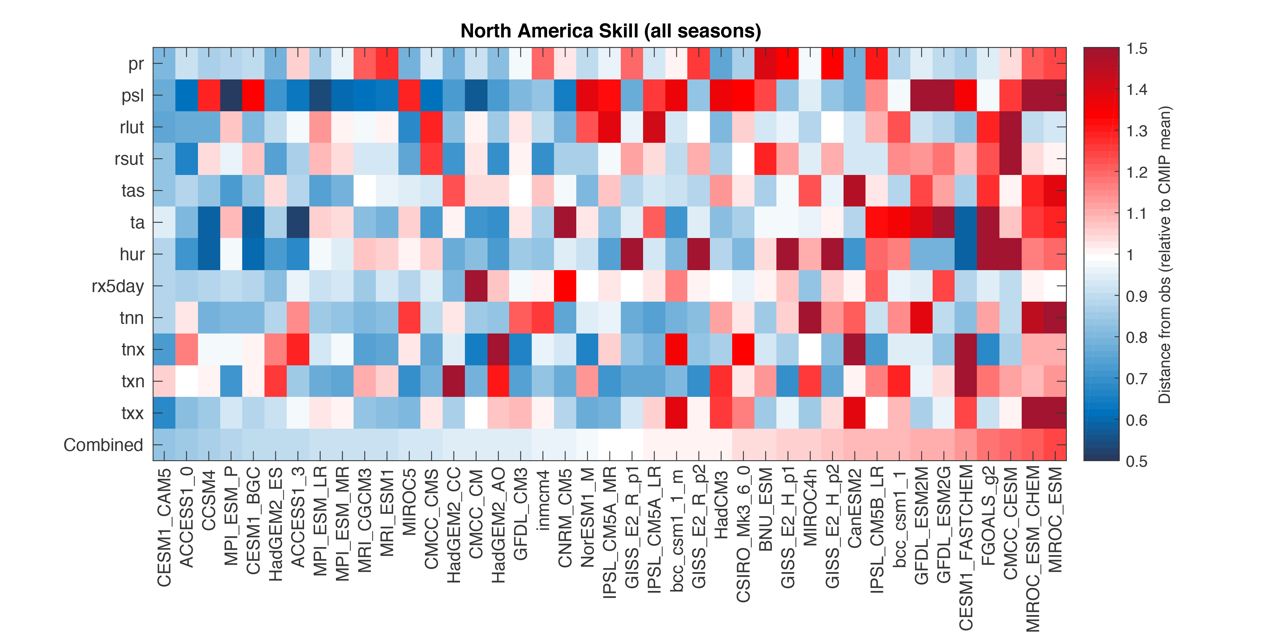
A graphical representation of the intermodel distance matrix for CMIP5 and a set of observed values. Each row and column represents a single climate model (or observation). All scores are aggregated over seasons (individual seasons are not shown). Each box represents a pairwise distance, where warm (red) colors indicate a greater distance. Distances are measured as a fraction of the mean intermodel distance in the CMIP5 ensemble. (Figure source: Sanderson et al. 20172 ).
Figure 2
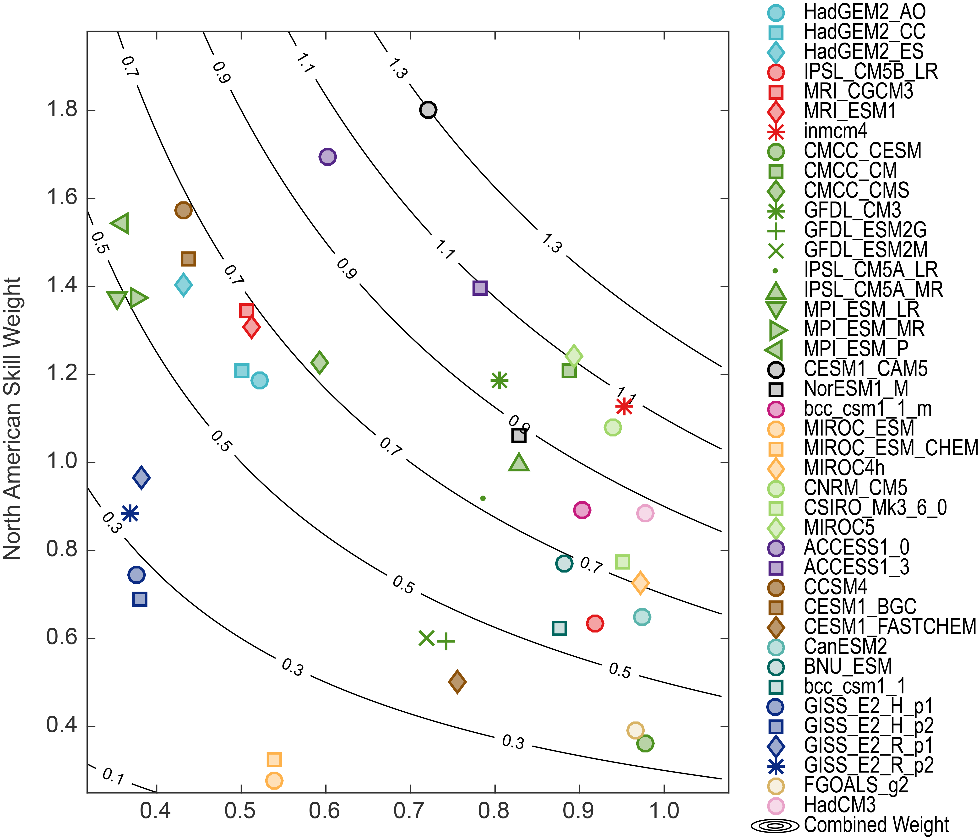
Model skill and independence weights for the CMIP5 archive evaluated over the North American domain. Contours show the overall weighting, which is the product of the two individual weights. (Figure source: Sanderson et al. 20172 ).
Models are downweighted for poor skill if their multivariate combined error is significantly greater than a “skill radius” term, which is a free parameter of the approach. The calibration of this parameter is determined through a perfect model study.2 A pairwise distance matrix is computed to assess intermodel RMSE values for each model pair in the archive, and a model is downweighted for dependency if there exists another model with a pairwise distance to the original model significantly smaller than a “similarity radius.” This is the second parameter of the approach, which is calibrated by considering known relationships within the archive. The resulting skill and independence weights are multiplied to give an overall “combined” weight—illustrated in Figure B.2 for the CMIP5 ensemble and listed in Table B.2.
The weights are used in the Climate Science Special Report (CSSR) to produce weighted mean and significance maps of future change, where the following protocol is used:
Stippling—large changes, where the weighted multimodel average change is greater than double the standard deviation of the 20-year mean from control simulations runs, and 90% of the weight corresponds to changes of the same sign.
Hatching—No significant change, where the weighted multimodel average change is less than the standard deviation of the 20-year means from control simulations runs.
Whited out—Inconclusive, where the weighted multimodel average change is greater than double the standard deviation of the 20-year mean from control runs and less than 90% of the weight corresponds to changes of the same sign.
Figure 3
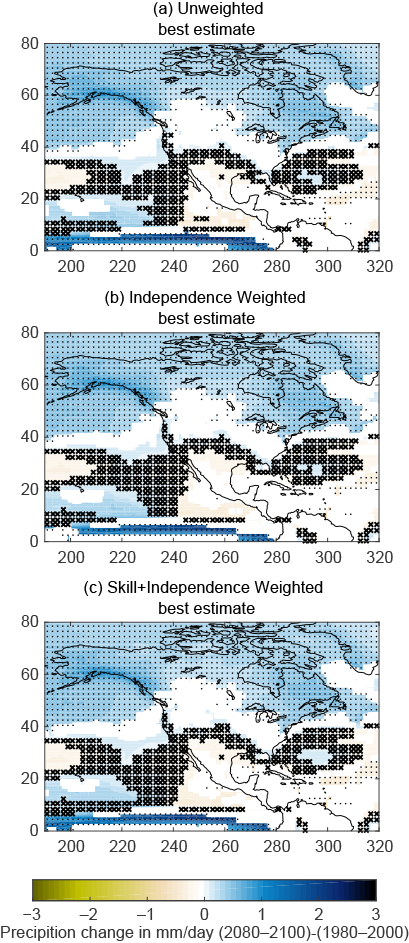
Projections of precipitation change over North America in 2080–2100, relative to 1980–2000 under the higher scenario (RCP8.5). (a) Shows the simple unweighted CMIP5 multimodel average, using the significance methodology from IPCC9 ; (b) shows the weighted results as outlined in Section 3 for models weighted by uniqueness only; and (c) shows weighted results for models weighted by both uniqueness and skill. (Figure source: Sanderson et al. 20172 ).
We illustrate the application of this method to future projections of precipitation change under the higher scenario (RCP8.5) in Figure B.3. The weights used in the report are chosen to be conservative, minimizing the risk of overconfidence and maximizing out-of-sample predictive skill for future projections. This results (as in Figure B.3) in only modest differences in the weighted and unweighted maps. It is shown in Sanderson et al. 20172 that a more aggressive weighting strategy, or one focused on a particular variable, tends to exhibit a stronger constraint on future change relative to the unweighted case. It is also notable that tradeoffs exist between skill and replication in the archive (evident in Figure B.2), such that the weighting for both skill and uniqueness has a compensating effect. As such, mean projections using the CMIP5 ensemble are not strongly influenced by the weighting. However, the establishment of the weighting strategy used in the CSSR provides some insurance against a potential case in future assessments where there is a highly replicated, but poorly performing model.
| Field | Description | Source | Reference | Years |
|---|---|---|---|---|
| TS | Surface Temperature (seasonal) | Livneh, Hutchinson | (Hopkinson et al. 2012;3 Hutchinson et al. 2009;4 Livneh et al. 20135 ) | 1950–2011 |
| PR | Mean Precipitation (seasonal) | Livneh, Hutchinson | (Hopkinson et al. 2012;3 Hutchinson et al. 2009;4 Livneh et al. 20135 ) | 1950–2011 |
| RSUT | TOA Shortwave Flux (seasonal) | CERES-EBAF | (Wielicki et al. 19966 ) | 2000–2005 |
| RLUT | TOA Longwave Flux (seasonal) | CERES-EBAF | (Wielicki et al. 19966 ) | 2000–2005 |
| T | Vertical Temperature Profile (seasonal) | AIRS* | (Aumann et al. 20037 ) | 2002–2010 |
| RH | Vertical Humidity Profile (seasonal) | AIRS | (Aumann et al. 20037 ) | 2002–2010 |
| PSL | Surface Pressure (seasonal) | ERA-40 | (Uppala et al. 20058 ) | 1970–2000 |
| Tnn | Coldest Night | Livneh, Hutchinson | (Hopkinson et al. 2012;3 Hutchinson et al. 2009;4 Livneh et al. 20135 ) | 1950–2011 |
| Txn | Coldest Day | Livneh, Hutchinson | (Hopkinson et al. 2012;3 Hutchinson et al. 2009;4 Livneh et al. 20135 ) | 1950–2011 |
| Tnx | Warmest Night | Livneh, Hutchinson | (Hopkinson et al. 2012;3 Hutchinson et al. 2009;4 Livneh et al. 20135 ) | 1950–2011 |
| Txx | Warmest day | Livneh, Hutchinson | (Hopkinson et al. 2012;3 Hutchinson et al. 2009;4 Livneh et al. 20135 ) | 1950–2011 |
| rx5day | seasonal max. 5-day total precip. | Livneh, Hutchinson | (Hopkinson et al. 2012;3 Hutchinson et al. 2009;4 Livneh et al. 20135 ) | 1950–2011 |
| Uniqueness Weight | Skill Weight | Combined | |
|---|---|---|---|
| ACCESS1-0 | 0.60 | 1.69 | 1.02 |
| ACCESS1-3 | 0.78 | 1.40 | 1.09 |
| BNU-ESM | 0.88 | 0.77 | 0.68 |
| CCSM4 | 0.43 | 1.57 | 0.68 |
| CESM1-BGC | 0.44 | 1.46 | 0.64 |
| CESM1-CAM5 | 0.72 | 1.80 | 1.30 |
| CESM1-FASTCHEM | 0.76 | 0.50 | 0.38 |
| CMCC-CESM | 0.98 | 0.36 | 0.35 |
| CMCC-CM | 0.89 | 1.21 | 1.07 |
| CMCC-CMS | 0.59 | 1.23 | 0.73 |
| CNRM-CM5 | 0.94 | 1.08 | 1.01 |
| CSIRO-Mk3-6-0 | 0.95 | 0.77 | 0.74 |
| CanESM2 | 0.97 | 0.65 | 0.63 |
| FGOALS-g2 | 0.97 | 0.39 | 0.38 |
| GFDL-CM3 | 0.81 | 1.18 | 0.95 |
| GFDL-ESM2G | 0.74 | 0.59 | 0.44 |
| GFDL-ESM2M | 0.72 | 0.60 | 0.43 |
| GISS-E2-H-p1 | 0.38 | 0.74 | 0.28 |
| GISS-E2-H-p2 | 0.38 | 0.69 | 0.26 |
| GISS-E2-R-p1 | 0.38 | 0.97 | 0.37 |
| GISS-E2-R-p2 | 0.37 | 0.89 | 0.33 |
| HadCM3 | 0.98 | 0.89 | 0.87 |
| HadGEM2-AO | 0.52 | 1.19 | 0.62 |
| HadGEM2-CC | 0.50 | 1.21 | 0.60 |
| HadGEM2-ES | 0.43 | 1.40 | 0.61 |
| IPSL-CM5A-LR | 0.79 | 0.92 | 0.72 |
| IPSL-CM5A-MR | 0.83 | 0.99 | 0.82 |
| IPSL-CM5B-LR | 0.92 | 0.63 | 0.58 |
| MIROC-ESM | 0.54 | 0.28 | 0.15 |
| MIROC-ESM-CHEM | 0.54 | 0.32 | 0.17 |
| MIROC4h | 0.97 | 0.73 | 0.71 |
| MIROC5 | 0.89 | 1.24 | 1.11 |
| MPI-ESM-LR | 0.35 | 1.38 | 0.49 |
| MPI-ESM-MR | 0.38 | 1.37 | 0.52 |
| MPI-ESM-P | 0.36 | 1.54 | 0.56 |
| MRI-CGCM3 | 0.51 | 1.35 | 0.68 |
| MRI-ESM1 | 0.51 | 1.31 | 0.67 |
| NorESM1-M | 0.83 | 1.06 | 0.88 |
| bcc-csm1-1 | 0.88 | 0.62 | 0.55 |
| bcc-csm1-1-m | 0.90 | 0.89 | 0.80 |
| inmcm4 | 0.95 | 1.13 | 1.08 |
References
- Aumann, H. H., M. T. Chahine, C. Gautier, M. D. Goldberg, E. Kalnay, L. M. McMillin, H. Revercomb, P. W. Rosenkranz, W. L. Smith, D. H. Staelin, L. L. Strow, and J. Susskind, 2003: AIRS/AMSU/HSB on the Aqua mission: Design, science objectives, data products, and processing systems. IEEE Transactions on Geoscience and Remote Sensing, 41, 253–264, doi:10.1109/TGRS.2002.808356. ↩
- Hopkinson, R. F., M. F. Hutchinson, D. W. McKenney, E. J. Milewska, and P. Papadopol, 2012: Optimizing input data for gridding climate normals for Canada. Journal of Applied Meteorology and Climatology, 51, 1508–1518, doi:10.1175/JAMC-D-12-018.1. ↩
- Hutchinson, M. F., D. W. McKenney, K. Lawrence, J. H. Pedlar, R. F. Hopkinson, E. Milewska, and P. Papadopol, 2009: Development and testing of Canada-wide interpolated spatial models of daily minimum–maximum temperature and precipitation for 1961–2003. Journal of Applied Meteorology and Climatology, 48, 725–741, doi:10.1175/2008JAMC1979.1. ↩
- IPCC, 2013: Climate Change 2013: The Physical Science Basis. Contribution of Working Group I to the Fifth Assessment Report of the Intergovernmental Panel on Climate Change. 1535 pp., Cambridge University Press. ↩
- Livneh, B., E. A. Rosenberg, C. Lin, B. Nijssen, V. Mishra, K. M. Andreadis, E. P. Maurer, and D. P. Lettenmaier, 2013: A long-term hydrologically based dataset of land surface fluxes and states for the conterminous United States: Update and extensions. Journal of Climate, 26, 9384–9392, doi:10.1175/JCLI-D-12-00508.1. ↩
- Sanderson, B. M., M. Wehner, and R. Knutti, 2017: Skill and independence weighting for multi-model assessment. Geoscientific Model Development, 10, 2379–2395, doi:10.5194/gmd-10-2379-2017. ↩
- Sanderson, B. M., R. Knutti, and P. Caldwell, 2015: A representative democracy to reduce interdependency in a multimodel ensemble. Journal of Climate, 28, 5171–5194, doi:10.1175/JCLI-D-14-00362.1. ↩
- Uppala, S. M. et al., 2005: The ERA-40 re-analysis. Quarterly Journal of the Royal Meteorological Society, 131, 2961–3012, doi:10.1256/qj.04.176. ↩
- Wielicki, B. A., B. R. Barkstrom, E. F. Harrison, R. B. Lee III, G. L. Smith, and J. E. Cooper, 1996: Clouds and the Earth’s Radiant Energy System (CERES): An Earth observing system experiment. Bulletin of the American Meteorological Society, 77, 853–868, doi:10.1175/1520-0477(1996)077<0853:catere>2.0.co;2. ↩