15.1: Introduction
The Earth system is made up of many components that interact in complex ways across a broad range of temporal and spatial scales. As a result of these interactions the behavior of the system cannot be predicted by looking at individual components in isolation. Negative feedbacks, or self-stabilizing cycles, within and between components of the Earth system can dampen changes (Ch. 2: Physical Drivers of Climate Change). However, their stabilizing effects render such feedbacks of less concern from a risk perspective than positive feedbacks, or self-reinforcing cycles. Positive feedbacks magnify both natural and anthropogenic changes. Some Earth system components, such as arctic sea ice and the polar ice sheets, may exhibit thresholds beyond which these self-reinforcing cycles can drive the component, or the entire system, into a radically different state. Although the probabilities of these state shifts may be difficult to assess, their consequences could be high, potentially exceeding anything anticipated by climate model projections for the coming century.
Humanity’s effect on the Earth system, through the large-scale combustion of fossil fuels and widespread deforestation and the resulting release of carbon dioxide (CO2) into the atmosphere, as well as through emissions of other greenhouse gases and radiatively active substances from human activities, is unprecedented (Ch. 2: Physical Drivers of Climate Change). These forcings are driving changes in temperature and other climate variables. Previous chapters have covered a variety of observed and projected changes in such variables, including averages and extremes of temperature, precipitation, sea level, and storm events (see Chapters 1, 4–13).
While the distribution of climate model projections provides insight into the range of possible future changes, this range is limited by the fact that models do not include or fully represent all of the known processes and components of the Earth system (e.g., ice sheets or arctic carbon reservoirs),1 nor do they include all of the interactions between these components that contribute to the self-stabilizing and self-reinforcing cycles mentioned above (e.g., the dynamics of the interactions between ice sheets, the ocean, and the atmosphere). They also do not include currently unknown processes that may become increasingly relevant under increasingly large climate forcings. This limitation is emphasized by the systematic tendency of climate models to underestimate temperature change during warm paleoclimates (Section 15.5). Therefore, there is significant potential for humanity’s effect on the planet to result in unanticipated surprises and a broad consensus that the further and faster the Earth system is pushed towards warming, the greater the risk of such surprises.
Scientists have been surprised by the Earth system many times in the past. The discovery of the ozone hole is a clear example. Prior to groundbreaking work by Molina and Rowland2 , chlorofluorocarbons (CFCs) were viewed as chemically inert; the chemistry by which they catalyzed stratospheric ozone depletion was unknown. Within eleven years of Molina and Rowland’s work, British Antarctic Survey scientists reported ground observations showing that spring ozone concentrations in the Antarctic, driven by chlorine from human-emitted CFCs, had fallen by about one-third since the late 1960s.3 The problem quickly moved from being an “unknown unknown” to a “known known,” and by 1987, the Montreal Protocol was adopted to phase out these ozone-depleting substances.
Another surprise has come from arctic sea ice. While the potential for powerful positive ice-albedo feedbacks has been understood since the late 19th century, climate models have struggled to capture the magnitude of these feedbacks and to include all the relevant dynamics that affect sea ice extent. As of 2007, the observed decline in arctic sea ice from the start of the satellite era in 1979 outpaced the declines projected by almost all the models used by the Intergovernmental Panel on Climate Change’s Fourth Assessment Report (AR4),4 and it was not until AR4 that the IPCC first raised the prospect of an ice-free summer Arctic during this century.5 More recent studies are more consistent with observations and have moved the date of an ice-free summer Arctic up to approximately mid-century (see Ch. 11: Arctic Changes).6 But continued rapid declines—2016 featured the lowest annually averaged arctic sea ice extent on record, and the 2017 winter maximum was also the lowest on record—suggest that climate models may still be underestimating or missing relevant feedback processes. These processes could include, for example, effects of melt ponds, changes in storminess and ocean wave impacts, and warming of near surface waters.7 ,8 ,9
This chapter focuses primarily on two types of potential surprises. The first arises from potential changes in correlations between extreme events that may not be surprising on their own but together can increase the likelihood of compound extremes, in which multiple events occur simultaneously or in rapid sequence. Increasingly frequent compound extremes—either of multiple types of events (such as paired extremes of droughts and intense rainfall) or over greater spatial or temporal scales (such as a drought occurring in multiple major agricultural regions around the world or lasting for multiple decades)—are often not captured by analyses that focus solely on one type of extreme.
The second type of surprise arises from self-reinforcing cycles, which can give rise to “tipping elements”—subcomponents of the Earth system that can be stable in multiple different states and can be “tipped” between these states by small changes in forcing, amplified by positive feedbacks. Examples of potential tipping elements include ice sheets, modes of atmosphere–ocean circulation like the El Niño–Southern Oscillation, patterns of ocean circulation like the Atlantic meridional overturning circulation, and large-scale ecosystems like the Amazon rainforest.10 ,11 While compound extremes and tipping elements constitute at least partially “known unknowns,” the paleoclimate record also suggests the possibility of “unknown unknowns.” These possibilities arise in part from the tendency of current climate models to underestimate past responses to forcing, for reasons that may or may not be explained by current hypotheses (e.g., hypotheses related to positive feedbacks that are unrepresented or poorly represented in existing models).
15.2: Risk Quantification and Its Limits
Quantifying the risk of low-probability, high-impact events, based on models or observations, usually involves examining the tails of a probability distribution function (PDF). Robust detection, attribution, and projection of such events into the future is challenged by multiple factors, including an observational record that often does not represent the full range of physical possibilities in the climate system, as well as the limitations of the statistical tools, scientific understanding, and models used to describe these processes.12
The 2013 Boulder, Colorado, floods and the Dust Bowl of the 1930s in the central United States are two examples of extreme events whose magnitude and/or extent are unprecedented in the observational record. Statistical approaches such as Extreme Value Theory can be used to model and estimate the magnitude of rare events that may not have occurred in the observational record, such as the “1,000-year flood event” (i.e., a flood event with a 0.1% chance of occurrence in any given year) (e.g., Smith 198713 ). While useful for many applications, these are not physical models: they are statistical models that are typically based on the assumption that observed patterns of natural variability (that is, the sample from which the models derive their statistics) are both valid and stationary beyond the observational period. Extremely rare events can also be assessed based upon paleoclimate records and physical modeling. In the paleoclimatic record, numerous abrupt changes have occurred since the last deglaciation, many larger than those recorded in the instrumental record. For example, tree ring records of drought in the western United States show abrupt, long-lasting megadroughts that were similar to but more intense and longer-lasting than the 1930s Dust Bowl.14
Since models are based on physics rather than observational data, they are not inherently constrained to any given time period or set of physical conditions. They have been used to study the Earth in the distant past and even the climate of other planets (e.g., Lunt et al. 2012;15 Navarro et al. 201416 ). Looking to the future, thousands of years’ worth of simulations can be generated and explored to characterize small-probability, high-risk extreme events, as well as correlated extremes (see Section 15.4). However, the likelihood that such model events represent real risks is limited by well-known uncertainties in climate modeling related to parameterizations, model resolution, and limits to scientific understanding (Ch. 4: Projections). For example, conventional convective parameterizations in global climate models systematically underestimate extreme precipitation.17 In addition, models often do not accurately capture or even include the processes, such as permafrost feedbacks, by which abrupt, non-reversible change may occur (see Section 15.4). An analysis focusing on physical climate predictions over the last 20 years found a tendency for scientific assessments such as those of the IPCC to under-predict rather than over-predict changes that were subsequently observed.18
15.3: Compound Extremes
An important aspect of surprise is the potential for compound extreme events. These can be events that occur at the same time or in sequence (such as consecutive floods in the same region) and in the same geographic location or at multiple locations within a given country or around the world (such as the 2009 Australian floods and wildfires). They may consist of multiple extreme events or of events that by themselves may not be extreme but together produce a multi-event occurrence (such as a heat wave accompanied by drought19 ). It is possible for the net impact of these events to be less than the sum of the individual events if their effects cancel each other out. For example, increasing CO2 concentrations and acceleration of the hydrological cycle may mitigate the future impact of extremes in gross primary productivity that currently impact the carbon cycle.20 However, from a risk perspective, the primary concern relates to compound extremes with additive or even multiplicative effects.
Some areas are susceptible to multiple types of extreme events that can occur simultaneously. For example, certain regions are susceptible to both flooding from coastal storms and riverine flooding from snow melt, and a compound event would be the occurrence of both simultaneously. Compound events can also result from shared forcing factors, including natural cycles like the El Niño–Southern Oscillation (ENSO); large-scale circulation patterns, such as the ridge observed during the 2011–2017 California drought (e.g., Swain et al. 201621 ; see also Ch. 8: Droughts, Floods, and Wildfires); or relatively greater regional sensitivity to global change, as may occur in “hot spots” such as the western United States.22 Finally, compound events can result from mutually reinforcing cycles between individual events, such as the relationship between drought and heat, linked through soil moisture and evaporation, in water-limited areas.23
In a changing climate, the probability of compound events can be altered if there is an underlying trend in conditions such as mean temperature, precipitation, or sea level that alters the baseline conditions or vulnerability of a region. It can also be altered if there is a change in the frequency or intensity of individual extreme events relative to the changing mean (for example, stronger storm surges, more frequent heat waves, or heavier precipitation events).
The occurrence of warm/dry and warm/wet conditions is discussed extensively in the literature; at the global scale, these conditions have increased since the 1950s,24 and analysis of NOAA’s billion-dollar disasters illustrates the correlation between temperature and precipitation extremes during the costliest climate and weather events since 1980 (Figure 15.1, right). In the future, hot summers will become more frequent, and although it is not always clear for every region whether drought frequency will change, droughts in already dry regions, such as the southwestern United States, are likely to be more intense in a warmer world due to faster evaporation and associated surface drying.25 ,26 ,27 For other regions, however, the picture is not as clear. Recent examples of heat/drought events (in the southern Great Plains in 2011 or in California, 2012–2016) have highlighted the inadequacy of traditional univariate risk assessment methods.28 Yet a bivariate analysis for the contiguous United States of precipitation deficits and positive temperature anomalies finds no significant trend in the last 30 years.29
Another compound event frequently discussed in the literature is the increase in wildfire risk resulting from the combined effects of high precipitation variability (wet seasons followed by dry), elevated temperature, and low humidity. If followed by heavy rain, wildfires can in turn increase the risk of landslides and erosion. They can also radically increase emissions of greenhouse gases, as demonstrated by the amount of carbon dioxide produced by the Fort McMurray fires of May 2016—more than 10% of Canada’s annual emissions.
A third example of a compound event involves flooding arising from wet conditions due to precipitation or to snowmelt, which could be exacerbated by warm temperatures. These wet conditions lead to high groundwater levels, saturated soils, and/or elevated river flows, which can increase the risk of flooding associated with a given storm days or even months later.23
Compound events may surprise in two ways. The first is if known types of compound events recur, but are stronger, longer-lasting, and/or more widespread than those experienced in the observational record or projected by model simulations for the future. One example would be simultaneous drought events in different agricultural regions across the country, or even around the world, that challenge the ability of human systems to provide adequate affordable food. Regions that lack the ability to adapt would be most vulnerable to this risk (e.g., Fraser et al. 201330 ). Another example would be the concurrent and more severe heavy precipitation events that have occurred in the U.S. Midwest in recent years. After record insurance payouts following the events, in 2014 several insurance companies, led by Farmers Insurance, sued the city of Chicago and surrounding counties for failing to adequately prepare for the impacts of a changing climate. Although the suit was dropped later that same year, their point was made: in some regions of the United States, the insurance industry is not able to cope with the increasing frequency and/or concurrence of certain types of extreme events.
The second way in which compound events could surprise would be the emergence of new types of compound events not observed in the historical record or predicted by model simulations, due to model limitations (in terms of both their spatial resolution as well as their ability to explicitly resolve the physical processes that would result in such compound events), an increase in the frequency of such events from human-induced climate change, or both. An example is Hurricane Sandy, where sea level rise, anomalously high ocean temperatures, and high tides combined to strengthen both the storm and the magnitude of the associated storm surge.31 At the same time, a blocking ridge over Greenland—a feature whose strength and frequency may be related to both Greenland surface melt and reduced summer sea ice in the Arctic (see also Ch. 11: Arctic Changes)32 —redirected the storm inland to what was, coincidentally, an exceptionally high-exposure location.
Figure 15.1
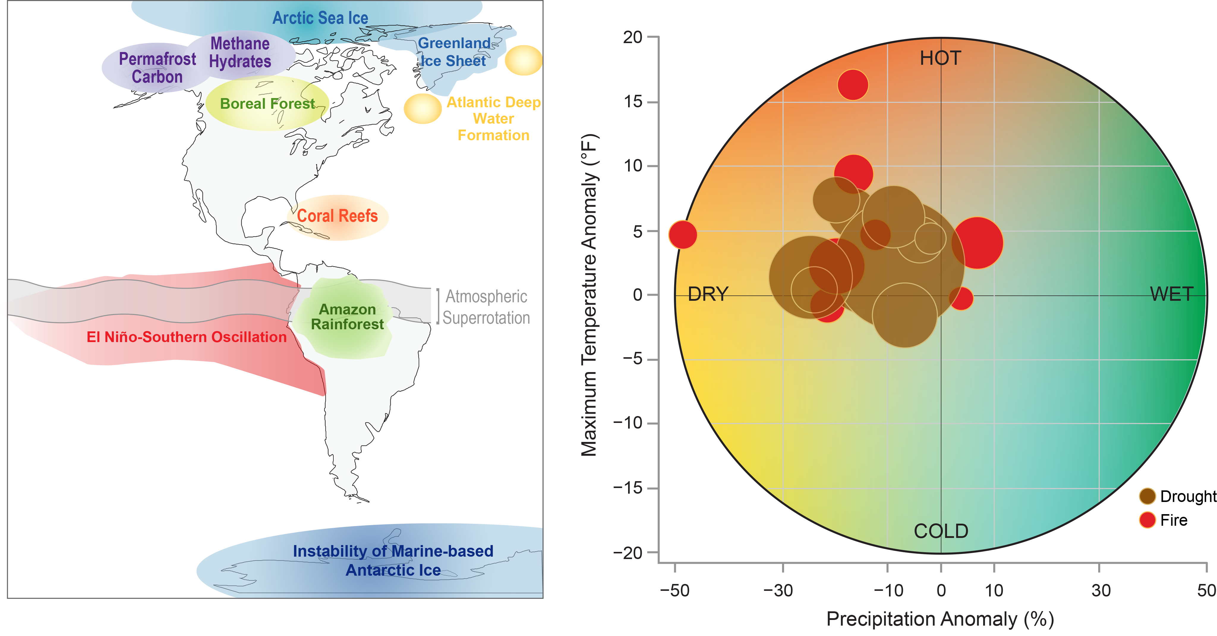
(left) Potential climatic tipping elements affecting the Americas (Figure source: adapted from Lenton et al. 200810 ). (right) Wildfire and drought events from the NOAA Billion Dollar Weather Events list (1980–2016), and associated temperature and precipitation anomalies. Dot size scales with the magnitude of impact, as reflected by the cost of the event. These high-impact events occur preferentially under hot, dry conditions.
15.4: Climatic Tipping Elements
Different parts of the Earth system exhibit critical thresholds, sometimes called “tipping points” (e.g., Lenton et al. 2008;10 Collins et al. 2013;25 NRC 2013;33 Kopp et al. 201611 ). These parts, known as tipping elements, have the potential to enter into self-amplifying cycles that commit them to shifting from their current state into a new state: for example, from one in which the summer Arctic Ocean is covered by ice, to one in which it is ice-free. In some potential tipping elements, these state shifts occur abruptly; in others, the commitment to a state shift may occur rapidly, but the state shift itself may take decades, centuries, or even millennia to play out. Often the forcing that commits a tipping element to a shift in state is unknown. Sometimes, it is even unclear whether a proposed tipping element actually exhibits tipping behavior. Through a combination of physical modeling, paleoclimate observations, and expert elicitations, scientists have identified a number of possible tipping elements in atmosphere–ocean circulation, the cryosphere, the carbon cycle, and ecosystems (Figure 15.1, left; Table 15.1).
| Candidate Climatic Tipping Element | State Shift | Main Impact Pathways |
|---|---|---|
| Atmosphere–ocean circulation | ||
| Atlantic meridional overturning circulation | Major reduction in strength | Regional temperature and precipitation; global mean temperature; regional sea level |
| El Niño–Southern Oscillation | Increase in amplitude | Regional temperature and precipitation |
| Equatorial atmospheric superrotation | Initiation | Cloud cover; climate sensitivity |
| Regional North Atlantic Ocean convection | Major reduction in strength | Regional temperature and precipitation |
| Cryosphere | ||
| Antarctic Ice Sheet | Major decrease in ice volume | Sea level; albedo; freshwater forcing on ocean circulation |
| Arctic sea ice | Major decrease in summertime and/or perennial area | Regional temperature and precipitation; albedo |
| Greenland Ice Sheet | Major decrease in ice volume | Sea level; albedo; freshwater forcing on ocean circulation |
| Carbon cycle | ||
| Methane hydrates | Massive release of carbon | Greenhouse gas emissions |
| Permafrost carbon | Massive release of carbon | Greenhouse gas emissions |
| Ecosystem | ||
| Amazon rainforest | Dieback, transition to grasslands | Greenhouse gas emissions; biodiversity |
| Boreal forest | Dieback, transition to grasslands | Greenhouse gas emissions; albedo; biodiversity |
| Coral reefs | Die-off | Biodiversity |
One important tipping element is the Atlantic meridional overturning circulation (AMOC), a major component of global ocean circulation. Driven by the sinking of cold, dense water in the North Atlantic near Greenland, its strength is projected to decrease with warming due to freshwater input from increased precipitation, glacial melt, and melt of the Greenland Ice Sheet (see also discussion in Ch. 11: Arctic Changes).34 A decrease in AMOC strength is probable and may already be culpable for the “warming hole” observed in the North Atlantic,34 ,35 although it is still unclear whether this decrease represents a forced change or internal variability.36 Given sufficient freshwater input, there is even the possibility of complete AMOC collapse. Most models do not predict such a collapse in the 21st century,33 although one study that used observations to bias-correct climate model simulations found that CO2 concentrations of 700 ppm led to a AMOC collapse within 300 years.37
A slowing or collapse of the AMOC would have several consequences for the United States. A decrease in AMOC strength would accelerate sea level rise off the northeastern United States,38 while a full collapse could result in as much as approximately 1.6 feet (0.5 m) of regional sea level rise,39 ,40 as well as a cooling of approximately 0°–4°F (0°–2°C) over the country.37 ,41 These changes would occur in addition to preexisting global and regional sea level and temperature change. A slowdown of the AMOC would also lead to a reduction of ocean carbon dioxide uptake, and thus an acceleration of global-scale warming.42
Another tipping element is the atmospheric–oceanic circulation of the equatorial Pacific that, through a set of feedbacks, drives the state shifts of the El Niño–Southern Oscillation. This is an example of a tipping element that already shifts on a sub-decadal, interannual timescale, primarily in response to internal noise. Climate model experiments suggest that warming will reduce the threshold needed to trigger extremely strong El Niño and La Niña events.43 ,44 As evident from recent El Niño and La Niña events, such a shift would negatively impact many regions and sectors across the United States (for more on ENSO impacts, see Ch. 5: Circulation and Variability).
A third potential tipping element is arctic sea ice, which may exhibit abrupt state shifts into summer ice-free or year-round ice-free states.45 ,46 As discussed above, climate models have historically underestimated the rate of arctic sea ice loss. This is likely due to insufficient representation of critical positive feedbacks in models. Such feedbacks could include: greater high-latitude storminess and ocean wave penetration as sea ice declines; more northerly incursions of warm air and water; melting associated with increasing water vapor; loss of multiyear ice; and albedo decreases on the sea ice surface (e.g., Schröder et al. 2014;7 Asplin et al. 2012;8 Perovich et al. 20089 ). At the same time, however, the point at which the threshold for an abrupt shift would be crossed also depends on the role of natural variability in a changing system; the relative importance of potential stabilizing negative feedbacks, such as more efficient heat transfer from the ocean to the atmosphere in fall and winter as sea declines; and how sea ice in other seasons, as well as the climate system more generally, responds once the first “ice-free” summer occurs (e.g., Ding et al. 201747 ). It is also possible that summer sea ice may not abruptly collapse, but instead respond in a manner proportional to the increase in temperature.48 ,49 ,50 ,51 Moreover, an abrupt decrease in winter sea ice may result simply as the gradual warming of Arctic Ocean causes it to cross a critical temperature for ice formation, rather than from self-reinforcing cycles.52
Two possible tipping elements in the carbon cycle also lie in the Arctic. The first is buried in the permafrost, which contains an estimated 1,300–1,600 GtC (see also Ch. 11: Arctic Changes).53 As the Arctic warms, about 5–15% is estimated to be vulnerable to release in this century.53 Locally, the heat produced by the decomposition of organic carbon could serve as a positive feedback, accelerating carbon release.54 However, the release of permafrost carbon, as well as whether that carbon is initially released as CO2 or as the more potent greenhouse gas CH4, is limited by many factors, including the freeze–thaw cycle, the rate with which heat diffuses into the permafrost, the potential for organisms to cycle permafrost carbon into new biomass, and oxygen availability. Though the release of permafrost carbon would probably not be fast enough to trigger a runaway self-amplifying cycle leading to a permafrost-free Arctic,53 it still has the potential to significantly amplify both local and global warming, reduce the budget of human-caused CO2 emissions consistent with global temperature targets, and drive continued warming even if human-caused emissions stopped altogether.55 ,56
The second possible arctic carbon cycle tipping element is the reservoir of methane hydrates frozen into the sediments of continental shelves of the Arctic Ocean (see also Ch. 11: Arctic Changes). There is an estimated 500 to 3,000 GtC in methane hydrates,57 ,58 ,59 with a most recent estimate of 1,800 GtC (equivalently, 2,400 Gt CH4).60 If released as methane rather than CO2, this would be equivalent to about 82,000 Gt CO2 using a global warming potential of 34.61 While the existence of this reservoir has been known and discussed for several decades (e.g., Kvenvolden 198862 ), only recently has it been hypothesized that warming bottom water temperatures may destabilize the hydrates over timescales shorter than millennia, leading to their release into the water column and eventually the atmosphere (e.g., Archer 2007;57 Kretschmer et al. 201563 ). Recent measurements of the release of methane from these sediments in summer find that, while methane hydrates on the continental shelf and upper slope are undergoing dissociation, the resulting emissions are not reaching the ocean surface in sufficient quantity to affect the atmospheric methane budget significantly, if at all.60 ,64 Estimates of plausible hydrate releases to the atmosphere over the next century are only a fraction of present-day anthropogenic methane emissions.60 ,63 ,65
These estimates of future emissions from permafrost and hydrates, however, neglect the possibility that humans may insert themselves into the physical feedback systems. With an estimated 53% of global fossil fuel reserves in the Arctic becoming increasingly accessible in a warmer world,66 the risks associated with this carbon being extracted and burned, further exacerbating the influence of humans on global climate, are evident.67 ,68 Of less concern but still relevant, arctic ocean waters themselves are a source of methane, which could increase as sea ice decreases.69
The Antarctic and Greenland Ice Sheets are clear tipping elements. The Greenland Ice Sheet exhibits multiple stable states as a result of feedbacks involving the elevation of the ice sheet, atmosphere-ocean-sea ice dynamics, and albedo.70 ,71 ,72 ,73 At least one study suggests that warming of 2.9ºF (1.6°C) above a preindustrial baseline could commit Greenland to an 85% reduction in ice volume and a 20 foot (6 m) contribution to global mean sea level over millennia.71 One 10,000-year modeling study74 suggests that following the higher RCP8.5 scenario (see Ch. 4: Projections) over the 21st century would lead to complete loss of the Greenland Ice Sheet over 6,000 years.
In Antarctica, the amount of ice that sits on bedrock below sea level is enough to raise global mean sea level by 75.5 feet (23 m).75 This ice is vulnerable to collapse over centuries to millennia due to a range of feedbacks involving ocean-ice sheet-bedrock interactions.74 ,76 ,77 ,78 ,79 ,80 Observational evidence suggests that ice dynamics already in progress have committed the planet to as much as 3.9 feet (1.2 m) worth of sea level rise from the West Antarctic Ice Sheet alone, although that amount is projected to occur over the course of many centuries.81 ,82 Plausible physical modeling indicates that, under the higher RCP8.5 scenario, Antarctic ice could contribute 3.3 feet (1 m) or more to global mean sea level over the remainder of this century,83 with some authors arguing that rates of change could be even faster.84 Over 10,000 years, one modeling study suggests that 3.6°F (2°C) of sustained warming could lead to about 70 feet (25 m) of global mean sea level rise from Antarctica alone.74
Finally, tipping elements also exist in large-scale ecosystems. For example, boreal forests such as those in southern Alaska may expand northward in response to arctic warming. Because forests are darker than the tundra they replace, their expansion amplifies regional warming, which in turn accelerates their expansion.85 As another example, coral reef ecosystems, such as those in Florida, are maintained by stabilizing ecological feedbacks among corals, coralline red algae, and grazing fish and invertebrates. However, these stabilizing feedbacks can be undermined by warming, increased risk of bleaching events, spread of disease, and ocean acidification, leading to abrupt reef collapse.86 More generally, many ecosystems can undergo rapid regime shifts in response to a range of stressors, including climate change (e.g., Scheffer et al. 2001;87 Folke et al. 200488 ).
15.5: Paleoclimatic Hints of Additional Potential Surprises
The paleoclimatic record provides evidence for additional state shifts whose driving mechanisms are as yet poorly understood. As mentioned, global climate models tend to underestimate both the magnitude of global mean warming in response to higher CO2 levels as well as its amplification at high latitudes, compared to reconstructions of temperature and CO2 from the geological record. Three case studies—all periods well predating the first appearance of Homo sapiens around 200,000 years ago89 —illustrate the limitations of current scientific understanding in capturing the full range of self-reinforcing cycles that operate within the Earth system, particularly over millennial time scales.
The first of these, the late Pliocene, occurred about 3.6 to 2.6 million years ago. Climate model simulations for this period systematically underestimate warming north of 30°N.90 During the second of these, the middle Miocene (about 17–14.5 million years ago), models also fail to simultaneously replicate global mean temperature—estimated from proxies to be approximately 14° ± 4°F (8° ± 2°C) warmer than preindustrial—and the approximately 40% reduction in the pole-to-equator temperature gradient relative to today.91 Although about one-third of the global mean temperature increase during the Miocene can be attributed to changes in geography and vegetation, geological proxies indicate CO2 concentrations of around 400 ppm,91 ,92 similar to today. This suggests the possibility of as yet unmodeled feedbacks, perhaps related to a significant change in the vertical distribution of heat in the tropical ocean.93
The last of these case studies, the early Eocene, occurred about 56–48 million years ago. This period is characterized by the absence of permanent land ice, CO2 concentrations peaking around 1,400 ± 470 ppm,94 and global temperatures about 25°F ± 5°F (14°C ± 3°C) warmer than the preindustrial.95 Like the late Pliocene and the middle Miocene, this period also exhibits about half the pole-to-equator temperature gradient of today.15 ,96 About one-third of the temperature difference is attributable to changes in geography, vegetation, and ice sheet coverage.95 However, to reproduce both the elevated global mean temperature and the reduced pole-to-equator temperature gradient, climate models would require CO2 concentrations that exceed those indicated by the proxy record by two to five times15 —suggesting once again the presence of as yet poorly understood processes and feedbacks.
One possible explanation for this discrepancy is a planetary state shift that, above a particular CO2 threshold, leads to a significant increase in the sensitivity of the climate to CO2. Paleo-data for the last 800,000 years suggest a gradual increase in climate sensitivity with global mean temperature over glacial-interglacial cycles,97 ,98 although these results are based on a time period with CO2 concentrations lower than today. At higher CO2 levels, one modeling study95 suggests that an abrupt change in atmospheric circulation (the onset of equatorial atmospheric superrotation) between 1,120 and 2,240 ppm CO2 could lead to a reduction in cloudiness and an approximate doubling of climate sensitivity. However, the critical threshold for such a transition is poorly constrained. If it occurred in the past at a lower CO2 level, it might explain the Eocene discrepancy and potentially also the Miocene discrepancy: but in that case, it could also pose a plausible threat within the 21st century under the higher RCP8.5 scenario.
Regardless of the particular mechanism, the systematic paleoclimatic model-data mismatch for past warm climates suggests that climate models are omitting at least one, and probably more, processes crucial to future warming, especially in polar regions. For this reason, future changes outside the range projected by climate models cannot be ruled out, and climate models are more likely to underestimate than to overestimate the amount of long-term future change.
References
- AghaKouchak, A., L. Cheng, O. Mazdiyasni, and A. Farahmand, 2014: Global warming and changes in risk of concurrent climate extremes: Insights from the 2014 California drought. Geophysical Research Letters, 41, 8847–8852, doi:10.1002/2014GL062308. ↩
- Anagnostou, E., E. H. John, K. M. Edgar, G. L. Foster, A. Ridgwell, G. N. Inglis, R. D. Pancost, D. J. Lunt, and P. N. Pearson, 2016: Changing atmospheric CO 2 concentration was the primary driver of early Cenozoic climate. Nature, 533, 380–384, doi:10.1038/nature17423. ↩
- Archer, D., 2007: Methane hydrate stability and anthropogenic climate change. Biogeosciences, 4, 521–544, doi:10.5194/bg-4-521-2007. ↩
- Armour, K. C., I. Eisenman, E. Blanchard-Wrigglesworth, K. E. McCusker, and C. M. Bitz, 2011: The reversibility of sea ice loss in a state-of-the-art climate model. Geophysical Research Letters, 38, L16705, doi:10.1029/2011GL048739. ↩
- Asplin, M. G., R. Galley, D. G. Barber, and S. Prinsenberg, 2012: Fracture of summer perennial sea ice by ocean swell as a result of Arctic storms. Journal of Geophysical Research, 117, C06025, doi:10.1029/2011JC007221. ↩
- Bathiany, S., D. Notz, T. Mauritsen, G. Raedel, and V. Brovkin, 2016: On the potential for abrupt Arctic winter sea ice loss. Journal of Climate, 29, 2703–2719, doi:10.1175/JCLI-D-15-0466.1. ↩
- Brysse, K., N. Oreskes, J. O’Reilly, and M. Oppenheimer, 2013: Climate change prediction: Erring on the side of least drama? Global Environmental Change, 23, 327–337, doi:10.1016/j.gloenvcha.2012.10.008. ↩
- Caballero, R., and M. Huber, 2013: State-dependent climate sensitivity in past warm climates and its implications for future climate projections. Proceedings of the National Academy of Sciences, 110, 14162–14167, doi:10.1073/pnas.1303365110. ↩
- Cai, W., G. Wang, A. Santoso, M. J. McPhaden, L. Wu, F.-F. Jin, A. Timmermann, M. Collins, G. Vecchi, M. Lengaigne, M. H. England, D. Dommenget, K. Takahashi, and E. Guilyardi, 2015: Increased frequency of extreme La Niña events under greenhouse warming. Nature Climate Change, 5, 132–137, doi:10.1038/nclimate2492. ↩
- Cai, W., S. Borlace, M. Lengaigne, P. van Rensch, M. Collins, G. Vecchi, A. Timmermann, A. Santoso, M. J. McPhaden, L. Wu, M. H. England, G. Wang, E. Guilyardi, and F.-F. Jin, 2014: Increasing frequency of extreme El Niño events due to greenhouse warming. Nature Climate Change, 4, 111–116, doi:10.1038/nclimate2100. ↩
- Cheng, J., Z. Liu, S. Zhang, W. Liu, L. Dong, P. Liu, and H. Li, 2016: Reduced interdecadal variability of Atlantic Meridional Overturning Circulation under global warming. Proceedings of the National Academy of Sciences, 113, 3175–3178, doi:10.1073/pnas.1519827113. ↩
- Clark, P. U. et al., 2016: Consequences of twenty-first-century policy for multi-millennial climate and sea-level change. Nature Climate Change, 6, 360–369, doi:10.1038/nclimate2923. ↩
- Collins, M., R. Knutti, J. Arblaster, J.-L. Dufresne, T. Fichefet, P. Friedlingstein, X. Gao, W. J. Gutowski, T. Johns, G. Krinner, M. Shongwe, C. Tebaldi, A. J. Weaver, and M. Wehner, 2013: Long-term climate change: Projections, commitments and irreversibility. T.F. Stocker, D. Qin, G.-K. Plattner, M. Tignor, S.K. Allen, J. Boschung, A. Nauels, Y. Xia, V. Bex, and P.M. Midgley, Eds., Cambridge University Press, 1029–1136. URL ↩
- Cook, B. I., T. R. Ault, and J. E. Smerdon, 2015: Unprecedented 21st century drought risk in the American Southwest and Central Plains. Science Advances, 1, e1400082, doi:10.1126/sciadv.1400082. ↩
- DeConto, R. M., and D. Pollard, 2016: Contribution of Antarctica to past and future sea-level rise. Nature, 531, 591–597, doi:10.1038/nature17145. ↩
- Diffenbaugh, N. S., and F. Giorgi, 2012: Climate change hotspots in the CMIP5 global climate model ensemble. Climatic Change, 114, 813–822, doi:10.1007/s10584-012-0570-x. ↩
- Ding, Q., A. Schweiger, M. Lheureux, D. S. Battisti, S. Po-Chedley, N. C. Johnson, E. Blanchard-Wrigglesworth, K. Harnos, Q. Zhang, R. Eastman, and E. J. Steig, 2017: Influence of high-latitude atmospheric circulation changes on summertime Arctic sea ice. Nature Climate Change, 7, 289–295, doi:10.1038/nclimate3241. ↩
- Drijfhout, S., G. J. van Oldenborgh, and A. Cimatoribus, 2012: Is a decline of AMOC causing the warming hole above the North Atlantic in observed and modeled warming patterns? Journal of Climate, 25, 8373–8379, doi:10.1175/jcli-d-12-00490.1. ↩
- Eisenman, I., and J. S. Wettlaufer, 2009: Nonlinear threshold behavior during the loss of Arctic sea ice. Proceedings of the National Academy of Sciences, 106, 28–32, doi:10.1073/pnas.0806887106. ↩
- Farman, J. C., B. G. Gardiner, and J. D. Shanklin, 1985: Large losses of total ozone in Antarctica reveal seasonal ClOx/NOx interaction. Nature, 315, 207–210, doi:10.1038/315207a0. ↩
- Flato, G., J. Marotzke, B. Abiodun, P. Braconnot, S. C. Chou, W. Collins, P. Cox, F. Driouech, S. Emori, V. Eyring, C. Forest, P. Gleckler, E. Guilyardi, C. Jakob, V. Kattsov, C. Reason, and M. Rummukainen, 2013: Evaluation of climate models. T.F. Stocker, D. Qin, G.-K. Plattner, M. Tignor, S.K. Allen, J. Boschung, A. Nauels, Y. Xia, V. Bex, and P.M. Midgley, Eds., Cambridge University Press, 741–866. URL ↩
- Folke, C., S. Carpenter, B. Walker, M. Scheffer, T. Elmqvist, L. Gunderson, and C. S. Holling, 2004: Regime shifts, resilience, and biodiversity in ecosystem management. Annual Review of Ecology, Evolution, and Systematics, 35, 557–581, doi:10.1146/annurev.ecolsys.35.021103.105711. ↩
- Foster, G. L., C. H. Lear, and J. W. B. Rae, 2012: The evolution of pCO 2 , ice volume and climate during the middle Miocene. Earth and Planetary Science Letters, 341–344, 243–254, doi:10.1016/j.epsl.2012.06.007. ↩
- Fraser, E. D. G., E. Simelton, M. Termansen, S. N. Gosling, and A. South, 2013: “Vulnerability hotspots”: Integrating socio-economic and hydrological models to identify where cereal production may decline in the future due to climate change induced drought. Agricultural and Forest Meteorology, 170, 195–205, doi:10.1016/j.agrformet.2012.04.008. ↩
- Fretwell, P. et al., 2013: Bedmap2: Improved ice bed, surface and thickness datasets for Antarctica. The Cryosphere, 7, 375–393, doi:10.5194/tc-7-375-2013. ↩
- Friedrich, T., A. Timmermann, M. Tigchelaar, O. Elison Timm, and A. Ganopolski, 2016: Nonlinear climate sensitivity and its implications for future greenhouse warming. Science Advances, 2, e1501923, doi:10.1126/sciadv.1501923. ↩
- G. Myhre, D. Shindell, F.-M. Bréon, W. Collins, J. Fuglestvedt, J. Huang, D. Koch, J.-F. Lamarque, D. Lee, B. Mendoza, T. Nakajima, A. Robock, G. Stephens, T. Takemura, and H. Zhang, 2013: Anthropogenic and natural radiative forcing. T.F. Stocker, D. Qin, G.-K. Plattner, M. Tignor, S.K. Allen, J. Boschung, A. Nauels, Y. Xia, V. Bex, and P.M. Midgley, Eds., Cambridge University Press, 659–740. URL ↩
- Goldner, A., N. Herold, and M. Huber, 2014: The challenge of simulating the warmth of the mid-Miocene climatic optimum in CESM1. Climate of the Past, 10, 523–536, doi:10.5194/cp-10-523-2014. ↩
- Gomez, N., J. X. Mitrovica, P. Huybers, and P. U. Clark, 2010: Sea level as a stabilizing factor for marine-ice-sheet grounding lines. Nature Geoscience, 3, 850–853, doi:10.1038/ngeo1012. ↩
- Gregory, J. M., and J. A. Lowe, 2000: Predictions of global and regional sea-level rise using AOGCMs with and without flux adjustment. Geophysical Research Letters, 27, 3069–3072, doi:10.1029/1999GL011228. ↩
- Hansen, J., M. Sato, P. Hearty, R. Ruedy, M. Kelley, V. Masson-Delmotte, G. Russell, G. Tselioudis, J. Cao, E. Rignot, I. Velicogna, B. Tormey, B. Donovan, E. Kandiano, K. von Schuckmann, P. Kharecha, A. N. Legrande, M. Bauer, and K. W. Lo, 2016: Ice melt, sea level rise and superstorms: Evidence from paleoclimate data, climate modeling, and modern observations that 2°C global warming could be dangerous. Atmospheric Chemistry and Physics, 16, 3761–3812, doi:10.5194/acp-16-3761-2016. ↩
- Hao, Z., A. AghaKouchak, and T. J. Phillips, 2013: Changes in concurrent monthly precipitation and temperature extremes. Environmental Research Letters, 8, 034014, doi:10.1088/1748-9326/8/3/034014. ↩
- Hoegh-Guldberg, O., P. J. Mumby, A. J. Hooten, R. S. Steneck, P. Greenfield, E. Gomez, C. D. Harvell, P. F. Sale, A. J. Edwards, K. Caldeira, N. Knowlton, C. M. Eakin, R. Iglesias-Prieto, N. Muthiga, R. H. Bradbury, A. Dubi, and M. E. Hatziolos, 2007: Coral reefs under rapid climate change and ocean acidification. Science, 318, 1737–1742, doi:10.1126/science.1152509. ↩
- Hollesen, J., H. Matthiesen, A. B. Møller, and B. Elberling, 2015: Permafrost thawing in organic Arctic soils accelerated by ground heat production. Nature Climate Change, 5, 574–578, doi:10.1038/nclimate2590. ↩
- Huber, M., and R. Caballero, 2011: The early Eocene equable climate problem revisited. Climate of the Past, 7, 603–633, doi:10.5194/cp-7-603-2011. ↩
- IPCC, 2012: Managing the Risks of Extreme Events and Disasters to Advance Climate Change Adaptation. A Special Report of Working Groups I and II of the Intergovernmental Panel on Climate Change. C.B. Field, V. Barros, T.F. Stocker, D. Qin, D.J. Dokken, K.L. Ebi, M.D. Mastrandrea, K.J. Mach, G.-K. Plattner, S.K. Allen, M. Tignor, and P.M. Midgley, Eds. Cambridge University Press, 582 pp. URL ↩
- Jackson, L. C., R. Kahana, T. Graham, M. A. Ringer, T. Woollings, J. V. Mecking, and R. A. Wood, 2015: Global and European climate impacts of a slowdown of the AMOC in a high resolution GCM. Climate Dynamics, 45, 3299–3316, doi:10.1007/s00382-015-2540-2. ↩
- Jakob, M., and J. Hilaire, 2015: Climate science: Unburnable fossil-fuel reserves. Nature, 517, 150–152, doi:10.1038/517150a. ↩
- Jones, C., J. Lowe, S. Liddicoat, and R. Betts, 2009: Committed terrestrial ecosystem changes due to climate change. Nature Geoscience, 2, 484–487, doi:10.1038/ngeo555. ↩
- Joughin, I., B. E. Smith, and B. Medley, 2014: Marine ice sheet collapse potentially under way for the Thwaites Glacier Basin, West Antarctica. Science, 344, 735–738, doi:10.1126/science.1249055. ↩
- Kang, I.-S., Y.-M. Yang, and W.-K. Tao, 2015: GCMs with implicit and explicit representation of cloud microphysics for simulation of extreme precipitation frequency. Climate Dynamics, 45, 325–335, doi:10.1007/s00382-014-2376-1. ↩
- Koenig, S. J., R. M. DeConto, and D. Pollard, 2014: Impact of reduced Arctic sea ice on Greenland ice sheet variability in a warmer than present climate. Geophysical Research Letters, 41, 3933–3942, doi:10.1002/2014GL059770. ↩
- Kopp, R. E., R. L. Shwom, G. Wagner, and J. Yuan, 2016: Tipping elements and climate–economic shocks: Pathways toward integrated assessment. Earth’s Future, 4, 346–372, doi:10.1002/2016EF000362. ↩
- Kort, E. A., S. C. Wofsy, B. C. Daube, M. Diao, J. W. Elkins, R. S. Gao, E. J. Hintsa, D. F. Hurst, R. Jimenez, F. L. Moore, J. R. Spackman, and M. A. Zondlo, 2012: Atmospheric observations of Arctic Ocean methane emissions up to 82° north. Nature Geoscience, 5, 318–321, doi:10.1038/ngeo1452. ↩
- Kretschmer, K., A. Biastoch, L. Rüpke, and E. Burwicz, 2015: Modeling the fate of methane hydrates under global warming. Global Biogeochemical Cycles, 29, 610–625, doi:10.1002/2014GB005011. ↩
- Kvenvolden, K. A., 1988: Methane hydrate — A major reservoir of carbon in the shallow geosphere? Chemical Geology, 71, 41–51, doi:10.1016/0009-2541(88)90104-0. ↩
- LaRiviere, J. P., A. C. Ravelo, A. Crimmins, P. S. Dekens, H. L. Ford, M. Lyle, and M. W. Wara, 2012: Late Miocene decoupling of oceanic warmth and atmospheric carbon dioxide forcing. Nature, 486, 97–100, doi:10.1038/nature11200. ↩
- Lee, S.-Y., and G. D. Holder, 2001: Methane hydrates potential as a future energy source. Fuel Processing Technology, 71, 181–186, doi:10.1016/S0378-3820(01)00145-X. ↩
- Lenton, T. M., H. Held, E. Kriegler, J. W. Hall, W. Lucht, S. Rahmstorf, and H. J. Schellnhuber, 2008: Tipping elements in the Earth’s climate system. Proceedings of the National Academy of Sciences, 105, 1786–1793, doi:10.1073/pnas.0705414105. ↩
- Levermann, A., A. Griesel, M. Hofmann, M. Montoya, and S. Rahmstorf, 2005: Dynamic sea level changes following changes in the thermohaline circulation. Climate Dynamics, 24, 347–354, doi:10.1007/s00382-004-0505-y. ↩
- Levermann, A., P. U. Clark, B. Marzeion, G. A. Milne, D. Pollard, V. Radic, and A. Robinson, 2013: The multimillennial sea-level commitment of global warming. Proceedings of the National Academy of Sciences, 110, 13745–13750, doi:10.1073/pnas.1219414110. ↩
- Li, C., D. Notz, S. Tietsche, and J. Marotzke, 2013: The transient versus the equilibrium response of sea ice to global warming. Journal of Climate, 26, 5624–5636, doi:10.1175/JCLI-D-12-00492.1. ↩
- Lindsay, R. W., and J. Zhang, 2005: The thinning of Arctic sea ice, 1988–2003: Have we passed a tipping point? Journal of Climate, 18, 4879–4894, doi:10.1175/jcli3587.1. ↩
- Liu, J., Z. Chen, J. Francis, M. Song, T. Mote, and Y. Hu, 2016: Has Arctic sea ice loss contributed to increased surface melting of the Greenland Ice Sheet? Journal of Climate, 29, 3373–3386, doi:10.1175/JCLI-D-15-0391.1. ↩
- Liu, W., S.-P. Xie, Z. Liu, and J. Zhu, 2017: Overlooked possibility of a collapsed Atlantic Meridional Overturning Circulation in warming climate. Science Advances, 3, e1601666, doi:10.1126/sciadv.1601666. ↩
- Lunt, D. J., T. Dunkley Jones, M. Heinemann, M. Huber, A. LeGrande, A. Winguth, C. Loptson, J. Marotzke, C. D. Roberts, J. Tindall, P. Valdes, and C. Winguth, 2012: A model–data comparison for a multi-model ensemble of early Eocene atmosphere–ocean simulations: EoMIP. Climate of the Past, 8, 1717–1736, doi:10.5194/cp-8-1717-2012. ↩
- MacDougall, A. H., C. A. Avis, and A. J. Weaver, 2012: Significant contribution to climate warming from the permafrost carbon feedback. Nature Geoscience, 5, 719–721, doi:10.1038/ngeo1573. ↩
- MacDougall, A. H., K. Zickfeld, R. Knutti, and H. D. Matthews, 2015: Sensitivity of carbon budgets to permafrost carbon feedbacks and non-CO 2 forcings. Environmental Research Letters, 10, 125003, doi:10.1088/1748-9326/10/12/125003. ↩
- McGlade, C., and P. Ekins, 2015: The geographical distribution of fossil fuels unused when limiting global warming to 2°C. Nature, 517, 187–190, doi:10.1038/nature14016. ↩
- Meehl, G. A., T. F. Stocker, W. D. Collins, P. Friedlingstein, A. T. Gaye, J. M. Gregory, A. Kitoh, R. Knutti, J. M. Murphy, A. Noda, S. C. B. Raper, I. G. Watterson, A. J. Weaver, and Z.-C. Zhao, 2007: Global Climate Projections. S. Solomon, D. Qin, M. Manning, Z. Chen, M. Marquis, K.B. Averyt, M. Tignor, and H.L. Miller, Eds., Cambridge University Press, 747–845. ↩
- Mengel, M., and A. Levermann, 2014: Ice plug prevents irreversible discharge from East Antarctica. Nature Climate Change, 4, 451–455, doi:10.1038/nclimate2226. ↩
- Molina, M. J., and F. S. Rowland, 1974: Stratospheric sink for chlorofluoromethanes: Chlorine atomc-atalysed destruction of ozone. Nature, 249, 810–812, doi:10.1038/249810a0. ↩
- Myhre, C. L. et al., 2016: Extensive release of methane from Arctic seabed west of Svalbard during summer 2014 does not influence the atmosphere. Geophysical Research Letters, 43, 4624–4631, doi:10.1002/2016GL068999. ↩
- NRC, 2013: Abrupt Impacts of Climate Change: Anticipating Surprises. The National Academies Press, 222 pp. ↩
- Navarro, T., J. B. Madeleine, F. Forget, A. Spiga, E. Millour, F. Montmessin, and A. Määttänen, 2014: Global climate modeling of the Martian water cycle with improved microphysics and radiatively active water ice clouds. Journal of Geophysical Research Planets, 119, 1479–1495, doi:10.1002/2013JE004550. ↩
- Perovich, D. K., J. A. Richter-Menge, K. F. Jones, and B. Light, 2008: Sunlight, water, and ice: Extreme Arctic sea ice melt during the summer of 2007. Geophysical Research Letters, 35, L11501, doi:10.1029/2008GL034007. ↩
- Piñero, E., M. Marquardt, C. Hensen, M. Haeckel, and K. Wallmann, 2013: Estimation of the global inventory of methane hydrates in marine sediments using transfer functions. Biogeosciences, 10, 959–975, doi:10.5194/bg-10-959-2013. ↩
- Pollard, D., R. M. DeConto, and R. B. Alley, 2015: Potential Antarctic Ice Sheet retreat driven by hydrofracturing and ice cliff failure. Earth and Planetary Science Letters, 412, 112–121, doi:10.1016/j.epsl.2014.12.035. ↩
- Pérez, F. F., H. Mercier, M. Vazquez-Rodriguez, P. Lherminier, A. Velo, P. C. Pardo, G. Roson, and A. F. Rios, 2013: Atlantic Ocean CO 2 uptake reduced by weakening of the meridional overturning circulation. Nature Geoscience, 6, 146–152, doi:10.1038/ngeo1680. ↩
- Quarantelli, E. L., 1986: Disaster Crisis Management. 10 pp., University of Delaware. URL ↩
- Rahmstorf, S., J. E. Box, G. Feulner, M. E. Mann, A. Robinson, S. Rutherford, and E. J. Schaffernicht, 2015: Exceptional twentieth-century slowdown in Atlantic Ocean overturning circulation. Nature Climate Change, 5, 475–480, doi:10.1038/nclimate2554. ↩
- Reed, A. J., M. E. Mann, K. A. Emanuel, N. Lin, B. P. Horton, A. C. Kemp, and J. P. Donnelly, 2015: Increased threat of tropical cyclones and coastal flooding to New York City during the anthropogenic era. Proceedings of the National Academy of Sciences, 112, 12610–12615, doi:10.1073/pnas.1513127112. ↩
- Ridley, J. K., J. A. Lowe, and H. T. Hewitt, 2012: How reversible is sea ice loss? The Cryosphere, 6, 193–198, doi:10.5194/tc-6-193-2012. ↩
- Ridley, J., J. M. Gregory, P. Huybrechts, and J. Lowe, 2010: Thresholds for irreversible decline of the Greenland ice sheet. Climate Dynamics, 35, 1049–1057, doi:10.1007/s00382-009-0646-0. ↩
- Rignot, E., J. Mouginot, M. Morlighem, H. Seroussi, and B. Scheuchl, 2014: Widespread, rapid grounding line retreat of Pine Island, Thwaites, Smith, and Kohler Glaciers, West Antarctica, from 1992 to 2011. Geophysical Research Letters, 41, 3502–3509, doi:10.1002/2014GL060140. ↩
- Ritz, C., T. L. Edwards, G. Durand, A. J. Payne, V. Peyaud, and R. C. A. Hindmarsh, 2015: Potential sea-level rise from Antarctic ice-sheet instability constrained by observations. Nature, 528, 115–118, doi:10.1038/nature16147. ↩
- Robinson, A., R. Calov, and A. Ganopolski, 2012: Multistability and critical thresholds of the Greenland ice sheet. Nature Climate Change, 2, 429–432, doi:10.1038/nclimate1449. ↩
- Ruppel, C. D., 2011: Methane hydrates and contemporary climate change. ↩
- Ruppel, C. D., and J. D. Kessler, 2017: The interaction of climate change and methane hydrates. Reviews of Geophysics, 55, 126–168, doi:10.1002/2016RG000534. ↩
- Salzmann, U. et al., 2013: Challenges in quantifying Pliocene terrestrial warming revealed by data-model discord. Nature Climate Change, 3, 969–974, doi:10.1038/nclimate2008. ↩
- Scheffer, M., S. Carpenter, J. A. Foley, C. Folke, and B. Walker, 2001: Catastrophic shifts in ecosystems. Nature, 413, 591–596, doi:10.1038/35098000. ↩
- Schoof, C., 2007: Ice sheet grounding line dynamics: Steady states, stability, and hysteresis. Journal of Geophysical Research, 112, F03S28, doi:10.1029/2006JF000664. ↩
- Schröder, D., D. L. Feltham, D. Flocco, and M. Tsamados, 2014: September Arctic sea-ice minimum predicted by spring melt-pond fraction. Nature Climate Change, 4, 353–357, doi:10.1038/nclimate2203. ↩
- Schuur, E. A. G., A. D. McGuire, C. Schadel, G. Grosse, J. W. Harden, D. J. Hayes, G. Hugelius, C. D. Koven, P. Kuhry, D. M. Lawrence, S. M. Natali, D. Olefeldt, V. E. Romanovsky, K. Schaefer, M. R. Turetsky, C. C. Treat, and J. E. Vonk, 2015: Climate change and the permafrost carbon feedback. Nature, 520, 171–179, doi:10.1038/nature14338. ↩
- Serinaldi, F., 2016: Can we tell more than we can know? The limits of bivariate drought analyses in the United States. Stochastic Environmental Research and Risk Assessment, 30, 1691–1704, doi:10.1007/s00477-015-1124-3. ↩
- Smith, J. A., 1987: Estimating the upper tail of flood frequency distributions. Water Resources Research, 23, 1657–1666, doi:10.1029/WR023i008p01657. ↩
- Stranne, C., M. O’Regan, G. R. Dickens, P. Crill, C. Miller, P. Preto, and M. Jakobsson, 2016: Dynamic simulations of potential methane release from East Siberian continental slope sediments. Geochemistry, Geophysics, Geosystems, 17, 872–886, doi:10.1002/2015GC006119. ↩
- Stroeve, J. C., V. Kattsov, A. Barrett, M. Serreze, T. Pavlova, M. Holland, and W. N. Meier, 2012: Trends in Arctic sea ice extent from CMIP5, CMIP3 and observations. Geophysical Research Letters, 39, L16502, doi:10.1029/2012GL052676. ↩
- Stroeve, J., M. M. Holland, W. Meier, T. Scambos, and M. Serreze, 2007: Arctic sea ice decline: Faster than forecast. Geophysical Research Letters, 34, L09501, doi:10.1029/2007GL029703. ↩
- Swain, D. L., D. E. Horton, D. Singh, and N. S. Diffenbaugh, 2016: Trends in atmospheric patterns conducive to seasonal precipitation and temperature extremes in California. Science Advances, 2, e1501344, doi:10.1126/sciadv.1501344. ↩
- Tattersall, I., 2009: Human origins: Out of Africa. Proceedings of the National Academy of Sciences, 106, 16018–16021, doi:10.1073/pnas.0903207106. ↩
- Trenberth, K. E., A. Dai, G. van der Schrier, P. D. Jones, J. Barichivich, K. R. Briffa, and J. Sheffield, 2014: Global warming and changes in drought. Nature Climate Change, 4, 17–22, doi:10.1038/nclimate2067. ↩
- Wagner, T. J. W., and I. Eisenman, 2015: How climate model complexity influences sea ice stability. Journal of Climate, 28, 3998–4014, doi:10.1175/JCLI-D-14-00654.1. ↩
- Woodhouse, C. A., and J. T. Overpeck, 1998: 2000 years of drought variability in the central United States. Bulletin of the American Meteorological Society, 79, 2693–2714, doi:10.1175/1520-0477(1998)079<2693:YODVIT>2.0.CO;2. ↩
- Yin, J., and P. B. Goddard, 2013: Oceanic control of sea level rise patterns along the East Coast of the United States. Geophysical Research Letters, 40, 5514–5520, doi:10.1002/2013GL057992. ↩
- Zscheischler, J., M. Reichstein, J. von Buttlar, M. Mu, J. T. Randerson, and M. D. Mahecha, 2014: Carbon cycle extremes during the 21st century in CMIP5 models: Future evolution and attribution to climatic drivers. Geophysical Research Letters, 41, 8853–8861, doi:10.1002/2014GL062409. ↩
- Zwiers, F. W., L. V. Alexander, G. C. Hegerl, T. R. Knutson, J. P. Kossin, P. Naveau, N. Nicholls, C. Schär, S. I. Seneviratne, and X. Zhang, 2013: Climate extremes: Challenges in estimating and understanding recent changes in the frequency and intensity of extreme climate and weather events. G.R. Asrar and J.W. Hurrell, Eds., Springer Netherlands, 339–389. ↩
- von der Heydt, A. S., P. Köhler, R. S. W. van de Wal, and H. A. Dijkstra, 2014: On the state dependency of fast feedback processes in (paleo) climate sensitivity. Geophysical Research Letters, 41, 6484–6492, doi:10.1002/2014GL061121. ↩